July 2017 – Cosmic Reflections

Apparent Magnitude, Absolute Magnitude, and Distance

A simple equation relates apparent magnitude, absolute magnitude, and distance. Know any two, and you can calculate the third.

Known: Apparent Magnitude (m), Absolute Magnitude (M)
Unknown: Distance (d), in parsecs

Known: Apparent Magnitude (m), Distance (d)
Unknown: Absolute Magnitude (M)

Known: Distance (d), Absolute Magnitude (M)
Unknown: Apparent Magnitude (m)

If this were a perfect universe, the known quantities could always be measured as precisely as one desires. But, of course, that isn’t the case.

Apparent Magnitude – if the observations are made from the surface of the Earth, atmospheric reddening and extinction (atmospheric r/e) must be taken into account to determine the apparent magnitude above the Earth’s atmosphere. Even above the Earth’s atmosphere, cosmic reddening and extinction (cosmic r/e) must also be quantified. Both atmospheric r/e and cosmic r/e¹ cause the observed apparent magnitude to appear fainter than it otherwise would be, and bluer wavelengths are more severely affected than redder wavelengths. The net result is to make objects appear fainter and redder than they would be if there were a perfect vacuum between source and observer.

Absolute Magnitude – is a measure of the intrinsic brightness of a celestial object, and this can only be measured indirectly for objects outside of our solar system.

Distance – is difficult to measure for objects outside of our solar system. Trigonometric parallax gives the most accurate results for nearby stars, but uncertainty increases rapidly with increasing distance.

Apparent magnitude is the only one of these quantities that is a direct instrumental measurement: absolute magnitude and distance are determined indirectly and thus are subject to greater uncertainty.

¹Atmospheric reddening and extinction (atmospheric r/e) is traditionally called atmospheric extinction, and cosmic reddening and extinction (cosmic r/e) is traditionally called interstellar reddening.  Since in both cases light is both reddened and diminished in intensity, and because "cosmic" encompasses both interstellar and intergalactic matter between source and observer, I suggest here that atmospheric r/e and cosmic r/e might be an improvement in terminology.

Milky Way Supernova Candidates

There is a supermassive binary star in our own Milky Way Galaxy that has the potential to create a super-supernova (hypernova?). It could go off tomorrow—or a million years from now. The star system’s name is Eta Carinae. Currently 4th-magnitude and located some 7,500 ly away in the direction of the southern constellation Carina (“The Keel”), Eta Carinae consists of a 100-200 M_☉ star and a 30-80 M_☉ star in a highly-eccentric 5.54^y orbit with the more massive star undergoing prodigious mass loss. Eta Carinae never rises above the horizon unless you’re south of latitude 30° N. So, if Eta Carina ever does go supernova while humans still walk the Earth, you’ll have to travel at least as far as southern Texas or southern Florida to see it. And it will be an impressive sight, easily visible during the daylight hours.

Closer to home, there are seven prime candidates for the next relatively nearby supernova. The nearest of these currently is IK Peg. Keep in mind that over hundreds of thousands of years, stars move quite a lot, so what is close to us now will not necessarily be close to us when a supernova event finally does occur.

IK Pegasi, a binary system comprised of a white dwarf already near the Chandrasekhar limit, and a close-by soon-to-be-giant main-sequence star, lies just 147 to 155 ly away in the direction of the constellation Pegasus, the Winged Horse. IK Peg appears to us visually as a 6th magnitude star located roughly ⅓ of the way from Delphinus to the Square of Pegasus. As the giant star expands into the vicinity of the white dwarf, the white dwarf will accumulate enough material to put it over the Chandrasekhar limit, and a Type Ia supernova will ensue.

Spica (α Vir), located at a distance between 237 and 264 ly, is a massive binary system (10 M_☉ and 7M_☉), with the two stars orbiting each other every four days.

Alpha Lupi (α Lup) is a massive star (~10 M_☉) located between 454 and 476 ly from our solar system.

Antares (α Sco) is a massive star (~12 M_☉, the supernova progenitor) orbited by another massive star (~7 M_☉). However, their orbital period is at least 1,200 years. The Antares system lies between 473 and 667 ly from our solar system

Betelgeuse (α Ori) is a massive star (~12 M_☉) between 500 and 900 ly away. Incidentally, there is a lot of uncertainty about the distance to Betelgeuse, primarily because it’s angular size (44 mas) is an order of magnitude larger than its parallax (4.5 mas) (Harper et al. 2017).

Rigel (β Ori) is a massive star (~23 M_☉) between 792 and 948 ly distant.

Gamma² Velorum (γ² Vel) is a binary system 1,013 to 1,245 ly distant containing two stars which will go supernova in the not-too-distant future. The system consists of a 28.5 M_☉O7.5 giant star and a 9.0 M_☉Wolf-Rayet star (the nearest, incidentally) orbiting each other every 78.5 days. The Wolf-Rayet star will be the first to supernova, followed later by the O giant star.

Tomorrow—or a million years from now? We have no way of accurately predicting. But rest assured, in the unlikely event that any one of these stars goes supernova during our lifetimes, none will be close enough to harm us. Instead, for a time, we will be treated to a object comparable to the Moon in brightness and visible both day and night.

References
Firestone, R.B., 2014, ApJ, 789, 29
Harper, G.M., Brown, A., Guinan, E.F., et al., 2017, AJ, 154, 11
Richardson, N.D., Russell, C.M.P., St-Jean, L., et al., 2017, MNRAS

Brightest Event Ever Observed

On June 14, 2015, perhaps the intrinsically brightest event ever recorded was detected at or near the center of the obscure galaxy APMUKS(BJ) B215839.70−615403.9 in the southern constellation Indus, at a luminosity distance of about 3.8 billion light years.

ASASSN-15lh (All–Sky Automated Survey for SuperNovae), also designated SN 2015L, is located at α₂₀₀₀=22^h02^m15.45^s, δ₂₀₀₀=-61° 39′ 34.6″ and is thought to be a super-luminous supernova—sometimes called a hypernova—but other interpretations are still in play.

Let’s put the brightness of SN 2015L in context. Peaking at an absolute visual magnitude of -24.925 (which would be its apparent visual magnitude at the standard distance of 10 parsecs), SN 2015L would shine as bright as the Sun in our sky if it were 14 light years away—about the distance to van Maanen’s Star, the nearest solitary white dwarf. SN 2015L would be as bright as the full moon if it were at a distance of 8,921 light years. SN 2015L would be as bright as the planet Venus if it were at a distance of 333,000 light years. Since the visible part of our galaxy is only about 100,000 ly across, had this supernova occurred anywhere in our galaxy, it would have been brighter than Venus. If SN 2015L had occurred in M31, the Andromeda Galaxy, 2.5 million light years away, it would take its place (albeit temporarily) as the third brightest star in the night sky (-0.47^m), after Sirius (-1.44^m) and Canopus (-0.62^m), but brighter than Alpha Centauri (-0.27^m) and Arcturus (-0.05^m).

The Open Supernova Catalog (Guillochon et al. 2017) lists three events that were possibly intrinsically brighter than SN 2015L. Two events were afterglows of gamma ray bursts GRB 81007 and GRB 30329: SN 2008hw at -25.014^m and SN 2003dh at -26.823^m, respectively. And the other event was the first supernova detected by the Gaia astrometric spacecraft, Gaia 14aaa, 500 Mly distant, shining perhaps as brightly as -27.1^m.

References
Chatzopoulos E., Wheeler J. C., Vinko J., et al., 2016, ApJ, 828, 94
Dong S., Shappee B. J., Prieto J. L., Jha S. W., et al., 2016, Science, 351, 257
Guillochon J., Parrent J., Kelley L. Z., Margutti R., 2017, ApJ, 835, 64

The Beginning

We continue our series of excerpts (and discussion) from the outstanding survey paper by George F. R. Ellis, Issues in the Philosophy of Cosmology.

Thesis D1: An initial singularity may or may not have occurred.
A start to the universe may have occurred a finite time ago, but a variety of alternatives are conceivable: eternal universes, or universes where time as we know it came into existence in one or another way. We do not know which actually happened, although quantum gravity ideas suggest a singularity might be avoided.

If we imagine, for a moment, running the clock of the universe backwards to earlier and earlier times, its size gets smaller and its density gets larger until we reach a moment—even earlier than the putative inflationary era—when classical physics at the macroscopic level no longer applies and some (as yet unknown) quantum physics must apply to everything—even gravity. Therein lies the problem, because if you run the clock backwards just 5.39 x 10^-44 second from this time, you reach the purported moment of the Big Bang—the initial singularity. But whoa (or perhaps woe)! How can we say anything about the Big Bang—or even if it occurred at all—since the laws of known physics completely break down 5.39 x 10^-44 second (the Planck time) after the Big Bang! See the problem?

Perhaps the universe came into existence through a process analogous to radioactive decay where an alpha particle leaves a nucleus through quantum tunneling. Perhaps our universe “tunneled” into existence from somewhere else, and thus our beginning isn’t really the beginning. This is just one of many possibilities.

This is a key issue in terms of the nature of the universe: a space-time singularity is a dramatic affair, where the universe (space, time, matter) has a beginning and all of physics breaks down and so the ability to understand what happens on a scientific basis comes to an end. However eternal existence is also problematic, leading for instance to the idea of Poincaré’s eternal return: everything that ever happened will recur an infinite number of times in the future and has already occurred an infinite number of times in the past. This is typical of the problems associated with the idea of infinity. It is not clear in the end which is philosophically preferable: a singularity or eternal existence. That decision will depend on what criteria of desirability one uses.

While infinity is a highly useful mathematical device, one can make a strong argument that infinities do not exist in the physical universe (or even multiverse). Quantum physics already gives us a possible clue about the infinitely small: we appear not to be able to subdivide space or time any further than the Planck length (1.616 x 10^-35 meter) or the Planck time (5.39 x 10^-44 second). We would not be able to distinguish between two points less than a Planck length apart, nor two moments in time less than a Planck time apart. While harder to envision, might not there also be an upper limit to size? And time?

Thesis D2: Testable physics cannot explain the initial state and hence specific nature of the universe.
A choice between different contingent possibilities has somehow occurred; the fundamental issue is what underlies this choice. Why does the universe have one specific form rather than another, when other forms consistent with physical laws seem perfectly possible? The reasons underlying the choice between different contingent possibilities for the universe (why one occurred rather than another) cannot be explored scientifically. It is an issue to be examined through philosophy or metaphysics.

Metaphysics is the part of philosophy that deals with existence, space, time, cause and effect, and the like. Metaphysics begins where physics necessarily ends due to observational limitations.

Did anything exist before the Big Bang?

Was there a Big Bang?

What are the physical properties of the very early universe, when energy densities existed that are far beyond our ability to recreate in the laboratory?

What lies beyond our particle horizon?

Are there other universes?

Why does anything exist at all?

References
Ellis, G. F. R. 2006, Issues in the Philosophy of Cosmology, Philosophy of Physics (Handbook of the Philosophy of Science), Ed. J. Butterfield and J. Earman (Elsevier, 2006), 1183-1285.
[http://arxiv.org/abs/astro-ph/0602280]

Liddle, A.R. 2015, An Introduction to Modern Cosmology, 3rd ed., Wiley, ISBN: 978-1-118-50214-3.

Where Voters Rejected Trump

The United States has never had a president like Donald Trump. And hopefully we will never have a president like him again. Regardless of your political persuasion, this man has neither the experience nor the temperament to be a public servant, and he should never have been elected.

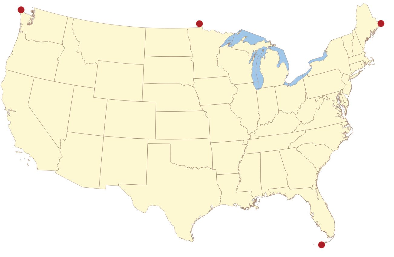
In the map below, you will find the 143 counties (or county equivalents) where Hillary Clinton received at least twice as many votes as Trump in the 2016 Presidential election. Counties in red have a lower population density than Iowa County, Wisconsin, and counties in blue a higher population density. Even though Iowa County, WI did not make the list, I am happy to say there were 1.39 Clinton voters for every Trump voter in this rural county in a state where Trump won (just barely) a majority of the votes.

Let us first look at the rural counties that voted heavily against Trump—by a 2 to 1 margin or better. All but 5 of the 40 rural counties have African-American, Hispanic, or Native American majorities.

The seventeen rural counties with African-American majorities (67.5% to 85.8%) are

Alabama
Bullock County
Greene County
Lowndes County
Perry County
Sumter County
Wilcox County

Georgia
Hancock County

Mississippi
Claiborne County
Holmes County
Humphreys County
Jefferson County
Noxubee County
Quitman County
Sharkey County
Tunica County
Wilkinson County

South Carolina
Allendale County

The per capita income in these counties with African-American majorities range from a low of $11,972 in Holmes County, Mississippi to $18,429 in Lowndes County, Alabama. The average for all seventeen counties is $14,344.

The twelve rural counties with Hispanic majorities (56.7% to 94.6%) are

New Mexico
Mora County
Rio Arriba County
San Miguel County
Taos County

Texas
Brooks County
Dimmit County
Duval County
Jim Hogg County
Presidio County
Willacy County
Zapata County
Zavala County

The per capita income in these counties with Hispanic majorities range from a low of $11,413 in Willacy County, Texas to $22,358 in Taos County, New Mexico. The average for all twelve counties is $17,171.

And the six rural counties with Native American majorities (75.4% to 92.8%) are

Arizona
Apache County

New Mexico
McKinley County

North Dakota
Sioux County

South Dakota
Oglala Lakota County
Todd County

Wisconsin
Menominee County

The per capita income in these counties with Native American majorities range from a low of $9,150 in Oglala Lakota County, South Dakota to $15,557 in Sioux County, North Dakota. The average for all six counties is $12,738.

Now let’s look at the five remaining rural counties that voted heavily against Trump in the 2016 general election.

California
Mendocino County

Colorado
Pitkin County
San Miguel County

Washington
Jefferson County
San Juan County

The per capita income in these counties range from a low of $24,059 in Mendocino County, California to $55,519 in Pitkin County, Colorado. The average for all five counties is $37,517.

Finally, here is a list of counties (and county equivalents) than have a higher population density than Iowa County, Wisconsin, where Hillary Clinton received at least twice as many votes as Donald Trump. These are listed by state, with the largest city in each county in parentheses.

Alabama
Dallas County (Selma)
Macon County (Tuskegee)

Arizona
Santa Cruz County (Nogales)

California
Alameda County (Oakland)
Contra Costa County (Concord)
Imperial County (El Centro)
Los Angeles County (Los Angeles)
Marin County (San Rafael)
Monterey County (Salinas)
Napa County (Napa)
San Francisco County (San Francisco)
San Mateo County (Daly City)
Santa Clara County (San Jose)
Santa Cruz County (Santa Cruz)
Sonoma County (Santa Rosa)
Yolo County (Davis)

Colorado
Boulder County (Boulder)
Denver County (Denver)

District of Columbia

Florida
Broward County (Fort Lauderdale)
Gadsden County (Quincy)

Georgia
Clarke County (Athens)
Clayton County (Forest Park)
DeKalb County (Brookhaven)
Dougherty County (Albany)
Fulton County (Atlanta)

Hawaii
Hawaii County (Hilo)
Kauai County (Kapaʻa)
Maui County (Kahului)

Illinois
Cook County (Chicago)

Iowa
Johnson County (Iowa City)

Kansas
Douglas County (Lawrence)

Louisiana
Orleans Parish (New Orleans)

Maryland
Howard County (Columbia)
Montgomery County (Germantown)
Prince George’s County (Bowie)
Baltimore City (Baltimore)

Massachusetts
Berkshire County (Pittsfield)
Dukes County (Edgartown)
Franklin County (Greenfield)
Hampshire County (Amherst)
Middlesex County (Lowell)
Nantucket County (Nantucket)
Suffolk County (Boston)

Michigan
Washtenaw County (Ann Arbor)
Wayne County (Detroit)

Minnesota
Hennepin County (Minneapolis)
Ramsey County (Saint Paul)

Mississippi
Coahoma County (Clarksdale)
Hinds County (Jackson)
Leflore County (Greenwood)
Sunflower County (Indianola)
Washington County (Greenville)

Missouri
St. Louis City (St. Louis)

New Jersey
Camden County (Camden)
Essex County (Newark)
Hudson County (Jersey City)
Mercer County (Hamilton Township)
Union County (Elizabeth)

New Mexico
Santa Fe County (Santa Fe)

New York
Bronx County (New York City: The Bronx)
Kings County (New York City: Brooklyn)
New York County (New York City: Manhattan)
Queens County (New York City: Queens)
Tompkins County (Ithaca)
Westchester County (Yonkers)

North Carolina
Durham County (Durham)
Hertford County (Ahoskie)
Orange County (Chapel Hill)

Ohio
Cuyahoga County (Cleveland)

Oregon
Benton County (Corvallis)
Multnomah County (Portland)

Pennsylvania
Philadelphia County (Philadelphia)

South Carolina
Orangeburg County (Orangeburg)
Richland County (Columbia)
Williamsburg County (Kingstree)

Texas
Cameron County (Brownsville)
El Paso County (El Paso)
Hidalgo County (McAllen)
Maverick County (Eagle Pass)
Starr County (Rio Grande City)
Travis County (Austin)
Webb County (Laredo)

Vermont
Addison County (Middlebury)
Chittenden County (Burlington)
Lamoille County (Morristown)
Washington County (Barre)
Windham County (Brattleboro)
Windsor County (Hartford)

Virginia
Arlington County (Arlington)
Fairfax County (Herndon)
Alexandria City (Alexandria)
Charlottesville City (Charlottesville)
Falls Church City (Falls Church)
Hampton City (Hampton)
Norfolk City (Norfolk)
Petersburg City (Petersburg)
Portsmouth City (Portsmouth)
Richmond City (Richmond)
Williamsburg City (Williamsburg)

Washington
King County (Seattle)

Wisconsin
Dane County (Madison)
Milwaukee County (Milwaukee)

References

Dave Leip’s Atlas of U.S. Presidential Elections, 2016 President County v1.0, 6-26-2017
United States Census Bureau, 2016 Population Estimates
United States Census Bureau, GCT-PH1 Population, Housing Units, Area, and Density: 2010 – United States — County by State; and for Puerto Rico
2010 Census Summary File 1
United States Census Bureau, QuickFacts V2016

Meteor Watching Site Needed Near Dodgeville

Meteor activity is starting to ramp up as we enter the second half of the year, and once again I am frustrated by those of us who live in Dodgeville not having a good location nearby for watching meteors. All that would be needed is a 12 x 12 ft. patch of ground that is kept mowed, has a good view of most of the sky, is not too near any cities or towns, and where no dusk-to-dawn insecurity lights are visible to spoil the view. Within about 10 miles of Dodgeville would be good, too, to minimize the late-night drive time home (and sleepy driving), especially on nights during the work week.

The Twin Valley Lake picnic area at Governor Dodge State Park is a perfect location for deploying a reclining lawn chair to watch meteors, but state park regulations prohibit such activities after 11:00 p.m. Most meteor showers are best after midnight, and this time of year when we’re on daylight saving time, 1:00 a.m. is really midnight.

I would even be willing to pay a monthly or per-use fee to a rural landowner for the privilege to set up my lawn chair on their land to watch meteors from time to time. Please add a comment here or email me at oesper at mac dot com to contact me about this.

In the Shadow of the Moon

Every once in a while a really great documentary comes along. In the Shadow of the Moon is one of them. This 2007 British film, which like most documentaries (unfortunately), had a very limited theater engagement, is now widely available for rental or purchase.

It is the remarkable story of the Apollo missions to the Moon, told eloquently by many of the astronauts who journeyed there: Buzz Aldrin, Michael Collins (Apollo 11), Alan Bean (Apollo 12), Jim Lovell (Apollo 8 & 13), Edgar Mitchell (Apollo 14), David Scott (Apollo 9 & 15), John Young (Apollo 10 & 16), Charles Duke (Apollo 16), Eugene Cernan (Apollo 10 & 17), and Harrison Schmitt (Apollo 17). You certainly get the impression that not only are these guys personable and intelligent, but that they have aged well and still have much insight and wisdom to offer us about the past, present, and future.

The historical importance of this documentary cannot be overstated. There is nothing, and I mean nothing, like hearing about the first (and still only) human missions to the Moon firsthand from the astronauts who journeyed there. And, sadly, these pioneering astronauts are not going to be with us much longer. Most have already left us. In the fourteen years since this documentary was released, Edgar Mitchell, the last surviving member of the Apollo 14 crew, passed away in 2016, Gene Cernan, the last man to walk on the Moon, passed away in 2017, John Young, the longest-serving astronaut in NASA history, and Alan Bean, the last surviving member of the Apollo 12 crew, left us in 2018, and Michael Collins passed away in 2021. The five surviving Apollo astronauts who shared their stories with us in this film are all octogenarians and nonagenarians: Jim Lovell is 93, Buzz Aldrin is 91, David Scott is 88, Charles Duke is 85, and Harrison Schmitt is 85.

This is a story that needed to be told by those who can tell it best. There is no narrator, nor is there any need for one. Kudos to directors David Sington & Christopher Riley, producers Duncan Copp, Christopher Riley, Sarah Kinsella, John Battsek, & Julie Goldman, and composer Philip Sheppard for making this a film of lasting cultural significance, a film that will be admired and appreciated a hundred-plus years from now.

Jupiter at Quadrature

Wednesday evening, July 5, around 9:40:17 p.m. CDT, Jupiter reaches east quadrature, which means it is 90° east of the Sun. In other words, the Sun-Earth-Jupiter line most nearly forms a right angle.

The best time to attempt daytime viewing of a superior planet like Jupiter is when it is at quadrature. Then, we are looking at it through a region of the sky where reflected sunlight is most strongly polarized. By using a polarizing filter with a telescope eyepiece, and properly rotating it, the sky background can be significantly darkened, allowing surprisingly good views of the planet during twilight and even daylight.

Jupiter reaches its most favorable viewing position when it crosses the celestial meridian, where it reaches its highest altitude, due south. Wednesday evening, that occurs at 6:58:18 p.m. (Dodgeville) when the Sun is 16° above the horizon, 1^h44^m before sunset. Use a polarizing filter for the best view of our solar system’s largest planet around this time on Wednesday, July 5—or the closest date that affords you clear skies.