The Lyman-alpha transition occurs when an electron in a hydrogen atom transitions from the first excited state (n=2) to the stable ground state (n=1), emitting an ultraviolet photon at 1215.67 Å. This and the other Lyman transitions to the ground state are named after American physicist and spectroscopist Theodore Lyman (1874-1954) who discovered and studied these spectral lines.
About 75% of the mass of our universe is hydrogen, so when we look at a very distant object, such as a quasar, the light from that distant object passes through a large number of tenuous hydrogen clouds between us and the distant object. The cooler hydrogen clouds absorb ultraviolet light at a wavelength of 1215.67 Å, so this wavelength is “removed” from the light from a distant object, as evinced by an absorption line in the spectrum of the distant object. But because the intervening neutral hydrogen clouds are moving at different speeds and cosmological redshifts, a number of different wavelengths have light removed (as seen from Earth), resulting in what is known as a Lyman-alpha forest. Analysis of the Lyman-alpha forest can tell us much about the neutral hydrogen clouds between us and any distant extragalactic source.
When a hydrogen cloud atom absorbs a 1215.67 Å ultraviolet photon, its electron jumps from the n=1 ground state up to the n=2 first excited state. However, excited electrons can’t stay in the n=2 state for long, and quickly return to the ground state again, emitting a photon of light at 1215.67 Å. So, why do we even see an absorption line? Yes, ultraviolet photons from the distant extragalactic source are removed from our line of sight by an intervening hydrogen cloud, but when ultraviolet photons are re-emitted, the photons radiate in all directions, and only a few travel towards us along our line of sight. The net result is an absorption line.
Even though the population of Dodgeville, Wisconsin is only around 4,800 people, there is quite a bit of traffic congestion along Dodgeville’s only real north-south through street: Iowa/Bequette, otherwise known as Wisconsin State Highway 23.
You’d never know it just driving through town, but the south part of WI 23 in Dodgeville is Iowa St. (S. Iowa St. south of Division St. and N. Iowa St. north of Division St.), and the north part of WI 23 is Bequette St., with the dividing line being Spring St., an unholy mess of an intersection that also includes Main St. and Diagonal St. (signed as Ohio St.). This is the perfect candidate for a roundabout if I ever saw one.
Making a left turn onto Iowa St. (which we often have to do) can be nerve-wracking with traffic, pedestrians, and in places poor visibility due to parked cars. A good way to solve this problem (and reduce the likelihood of accidents) would be to have one intersection along Iowa St. that has a traffic light. I think the ideal location for a traffic light would be the intersection of N. Iowa St. and Merrimac St.
Our current best estimate for the age of the universe (as we know it) is 13.799 Gyr ± 21 Myr. The Great Flaring Forth (GFF) occurred 13.8 billion years ago, and the universe has been expanding and cooling ever since.
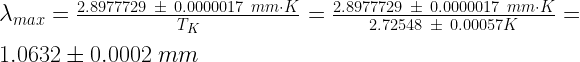
The background temperature of the universe is today 2.72548 ± 0.00057 K. “K” stands for Kelvin, a unit of temperature named after William Thomson, 1st Baron Kelvin (1824-1907) – Lord Kelvin – who championed the idea of an “absolute thermometric scale”. A temperature in Kelvin is equivalent to the number of Celsius degrees above absolute zero. Put into terms we may be more familiar with, the cosmic background temperature is -270.42452° C, or -454.764136° F. While in the absence of nearby stars or other energy sources, the universe is certainly cold, scientists have artificially produced temperatures as low as 100 pK (1 picoKelvin = 10-12 K).
Using Wien’s displacement law, we can calculate the wavelength of electromagnetic radiation where the background universe is brightest.
So, we see here that the background universe is “brightest” in the microwave part of the radio spectrum, at a peak wavelength around 1 mm. Using the relationship between frequency and wavelength, c = νλ, we can determine the microwave frequency where the background universe is brightest.
Microwaves at this frequency are in the extremely high frequency (EHF) radio band, above all our allocated communications bands (275-3000 GHz is unallocated).
Of course, a significant amount of emission occurs either side of the peak, particularly at longer wavelengths and lower frequencies. (The background universe radiates with an almost perfect blackbody spectrum.)
There are several ways to define the wavelength/frequency of maximum brightness. The above is one. Depending on the method we choose, the peak wavelength lies between 1.0623 and 3.313 mm, and the peak frequency between 90.5 and 282.0 GHz.
Wouldn’t it be nice if you got to choose where some of your income tax money goes? Where you the taxpayer have some say in how your hard-earned tax dollars are allocated?
Here in the dis-United States, about 50% of us want lower taxes, and 50% of us would be receptive to higher taxes provided that it pays for things we believe in like universal health care and low-cost or no-cost education.
Short of amicably splitting up our country (a civil separation), changing our tax policy may help alleviate some of the frustration many of us have that half of the country is keeping us from building the kind of country we want for ourselves and for our children.
Federal income tax, and state and local income tax (where in effect) would be divided into a non-discretionary portion (100% currently) and a discretionary portion.
When you fill out your tax return each year, you would designate the government agencies and programs where you want the discretionary portion of your taxes to go.
Going one step further, I would like to see taxpayers given the option to choose either the standard or a supplemental tax tier. Those who opt to pay higher taxes by choosing the supplemental tax tier would pay a fixed percentage more, regardless of income (like a true flat tax).
To be fair, those paying in at the higher supplemental tax rate should receive additional benefits compared to those paying in at the standard rate. This could mean lower medical costs, lower education costs, or increased social security payments during retirement, for example.
Would this be easier to implement than partitioning the U.S.? Perhaps. Would it be the more effective solution to satisfy those with very different viewpoints about the proper role of government? Perhaps not.
In my view, society is far too reliant on volunteers. If a job is worth doing, and if it is a benefit to society, then, more often than not, it needs to be a paid position. There is so much work of a humanitarian, educational, and environmental nature that needs to be done that cannot and will not be done by any capitalistic enterprise. As members of society, we all have an obligation to help fund these activities through strong government and non-sectarian non-profit partnerships.
I dream of a day when paying for our medical care is no longer tied to having health insurance through an employer, when each of us will have the freedom to work in a variety of capacities, for both profit and non-profit organizations, throughout our careers, and to receive adequate training and pay for those efforts.
Over five thousand years ago, the Sumerians in the area now known as southern Iraq appear to have been the first to develop a penchant for the numbers 12, 24, 60 and 360.
It is easy to see why. 12 is the first number that is evenly divisible by six smaller numbers:
12 = 1×12, 2×6, 3×4 .
24 is the first number that is evenly divisible by eight smaller numbers:
24 = 1×24, 2×12, 3×8, 4×6 .
60 is the first number than is evenly divisible by twelve smaller numbers:
60 = 1×60, 2×30, 3×20, 4×15, 5×12, 6×10 .
And 360 is the first number that is evenly divisible by twenty-four smaller numbers:
And 360 in a happy coincidence is just 1.4% short of the number of days in a year.
We have 12 hours in the morning, 12 hours in the evening.
We have 24 hours in a day.
We have 60 seconds in a minute, and 60 minutes in an hour.
We have 60 arcseconds in an arcminute, 60 arcminutes in a degree, and 360 degrees in a circle.
The current equatorial coordinates for the star Vega are
α2019.1 = 18h 37m 33s
δ2019.1 = +38° 47′ 58″
Due to precession, the right ascension (α) of Vega is currently increasing by 1s (one second of time) every 37 days, and its declination (δ) is currently decreasing by 1″ (one arcsecond) every 5 days.
With right ascension, the 360° in a circle is divided into 24 hours, therefore 1h is equal to (360°/24h) = 15°. Since there are 60 minutes in an hour and 60 seconds in a minute, and 60 arcminutes in a degree and 60 arcseconds in an arcminute, it follows that 1m = 15′ and 1s = 15″.
Increasingly, you will see right ascension and declination given in decimal, rather than sexagesimal, units. For Vega, currently, this would be
α2019.1 = 18.62583h δ2019.1 = +38.7994°
Or, both in degrees
α2019.1 = 279.3875° δ2019.1 = +38.7994°
Or even radians
α2019.1 = 4.876232 rad δ2019.1 = 0.677178 rad
Even though the latter three forms lend themselves well to computation, I still prefer the old sexagesimal form for “display” purposes, and when entering coordinates for “go to” at the telescope.
There is something aesthetically appealing about three sets of two-digit numbers, and, I think, this form is more easily remembered from one moment to the next.
For the same reason, we still use the sexagesimal form for timekeeping. For example, as I write this the current time is 12:25:14 a.m. which is a more attractive (and memorable) way to write the time than saying it is 12.4206 a.m. (unless you are doing computations).
That’s quite an achievement, developing something that is still in common use 5,000 years later.
About 80% of all known white dwarf stars have hydrogen atmospheres, showing only hydrogen absorption lines in their spectra. These have been assigned the white dwarf spectral type of DA (presumably D for dwarf and A for the first, or most common, type of white dwarf). Arlo Landolt (1935-) was the first to discover variability in a white dwarf by observing the mv=15.0 DA white dwarf star named HL Tau 76 (not to be confused with HL Tau!), in front of a dark nebula in Taurus (LDN 1521C = MLB 3-13), in December 1964. This star now has the standard variable star designation V411 Tauri.
A second DA white dwarf, mv=14.2 Ross 548 in Cetus, was discovered to be variable by Barry Lasker (1939-1999) and Jim Hesser in 1970, and in 1972 it was assigned the variable star designation ZZ Ceti.
By 1976, seven luminosity-variable DA white dwarfs had been discovered, and John T. McGraw and Edward L. Robinson stated in an ApJ paper
We suggest that the recently proposed ZZ Ceti class of variable stars be reserved for the DA variables in Table 1 and specifically exclude the DB variables since the mechanism of variation is almost certainly different.
McGraw & Robinson, Astrophysical Journal, Vol. 205, p. L155-L158 (1976)
So, why wasn’t this new class of luminosity-variable DA white dwarfs named after V411 Tau, the first of its class discovered? Why are they called ZZ Ceti stars, after the second such star discovered, instead? In each constellation, variable stars are given one- or two-letter designations in order of discovery, and when the letter designations run out, the letter “V” is used followed by a number. The first “V” star is V335, the 335th variable star to be discovered in a constellation. Well, V411 Tau was the 411th variable star discovered in Taurus, and as a matter of tradition, no class of variable stars is ever named after a “V” designation. So, the honor fell to the runner-up, ZZ Ceti. Besides, ZZ Cet is a little brighter than V411 Tau, so not a bad choice.
ZZ Ceti stars, also known as DAV stars (as in DA Variable), are multimodal pulsating white dwarfs having periods ranging from 70 seconds to 25 minutes. But the amplitude of the brightness variations is tiny to small, ranging from less than 0.001 magnitude up to 0.3 magnitudes.
V411 Tau has a dozen detected pulsation modes. In order of amplitude (in millimagnitudes), they are (without error bars):
Period (seconds)
Amplitude (mmag)
540.95
30.89
382.47
17.88
664.21
16.22
596.79
15.63
1064.97
12.27
781.0
9.88
492.12
7.73
449.8
7.27
976.38
7.01
799.10
5.63
1390.84
4.26
933.64
2.61
ZZ Cet has eleven detected pulsation modes. In order of amplitude, they are (without error bars):
Period (seconds)
Amplitude (mmag)
213.1326
7.119
274.2508
4.658
212.7684
4.448
274.7745
3.368
212.9463
1.477
274.5209
1.253
186.8740
0.9518
318.0763
0.7836
333.6447
0.6740
217.8336
0.3506
318.7657
0.3289
ZZ Ceti stars are not radial pulsators, that is they do not undergo radial oscillations (changes in size). White dwarf stars typically have diameters of only 0.9 to 2.2 that of the Earth, so they are much smaller than “normal” stars. As short as the pulsation periods are, they are not short enough if the cause were radial pulsations. Instead, the pulsations are due to shock waves traversing the atmosphere of the ultradense star. The slow rotation of these stars often causes closely spaced “double periods” such as we see in ZZ Cet.
The brightest (and closest) ZZ Ceti star yet discovered is DN Draconis, shining at visual magnitude 12.2. DN Dra pulsates with an amplitude of just 0.006 magnitude (6 millimagnitudes), and its pulsation period is 109 seconds.
What ZZ Ceti star has the largest amplitude? As they say, “it’s complicated”. Even though references to a maximum amplitude as high as 0.3m can be found in the literature, I was unable to find any ZZ Ceti stars with amplitudes greater than 0.12m. Moreover, pulsation modes of ZZ Ceti stars can come and go, so one observer may observe a higher amplitude but the next may not. Though pulsation modes can and do appear and disappear over time, there is also the changing additive nature of many pulsation modes to consider from one observing run to the next.
Patterson et. al (1991) report mv=13.0 ZZ Psc having a pulsation amplitude of 0.116m and period 614.9s in blue light. Mukadam et al. (2004) report mv=15.2 UCAC4 448-059643 (in the constellation Serpens) having a pulsation amplitude of 0.121m and period 873.2s in blue light.
One challenge in the literature is that pulsation amplitudes are variously given in units of milli-modulation amplitude (mma), milli-magnitudes (mmag), percent, or parts per thousand. Here are the unit conversions:
The study of the pulsation modes of white dwarfs and other stars is called asteroseismology. I hope this article has piqued your interest in learning more about this rapidly developing and fascinating field!
References Bognár, Z., Sódor, Á. 2016, Information Bulletin on Variable Stars,6184 Castanheira, B. G. & Kepler, S. O. 2008, MNRAS, 385, 430 De Gerónimo, F. C., Althaus, L. G., Córsico, et al. 2017, A&A, 599, A21 Dolez, N., Vauclair, G., Kleinman, S. J., et al. 2006, A&A, 446,237 Giammichele, N., Fontaine, G., Bergeron, P., et al. 2015, ApJ, 815, 56 Haro, G., and Luyten, W. J. 1961, Bol. Obs. Tonantzintlay Tacubaya, 3, 35 Kepler, S. O., Robinson, E. L., Koester, D., et al. 2000, ApJ, 539, 379 Kukarkin, B. V., Kholopov, P. N., Kukarkina, N. P., et al. 1972, IBVS, 717, 1 Landolt, A. U. 1968, ApJ, 153, 151 Lasker, B. M. & Hesser, J. E., 1971, ApJ, 163, L89 Lynds, B. T. 1962, ApJS, 7, 1 McGraw J. T. & Robinson E. L., 1976, ApJ, 205, L155 Mukadam, A. S., Mullally, F., Nather, R. E., et al. 2004, ApJ,607, 982 Myers, P. C., Linke, R. A., & Benson, P. J. 1983, ApJ, 264,517 Patterson, J., Zuckerman, B., Becklin E. E., et al. 1991, ApJ, 374, 330
The coldest weather I’ve ever experienced occurred January 30-31, 2019. Here in Dodgeville, Wisconsin, I measured a low temperature the morning of Wednesday, January 30, 2019 of -31.0° F and a high that day of -14.4° F. It was even colder the following night. On Thursday, January 31, 2019 the low temperature was -31.9° F.
Thanks to the National Weather Service, we had advance notice of the arrival of the Arctic polar vortex that was to bring the coldest weather to Wisconsin in a generation. Concerned about the effect this would have on my observatory electronics, I started running my warming room electric heater continuously from 8:30 p.m. CST Monday, January 28 until 9:45 a.m. CST Friday, February 1. Of course, I left the warming room door open to the telescope room to ensure that some of the heat would reach the telescope and its associated electronics.
During this time, I made a number of temperature measurements from an Oregon Scientific weather station inside the house, connected by 433 MHz radio frequency signals to temperature sensors inside the observatory and on the north side of my house.
And here is graph plotting both temperatures at each time:
Air (north side of house) and Observatory (inside the observatory) temperatures January 28-February 1, 2019.
And here is a plot of the temperature difference vs. the outside Air temperature:
Temperature difference vs. Air temperature with a linear regression line
There seems to be a general trend that the colder it was outside the observatory, the bigger was the temperature difference between inside the observatory and outside the observatory. Why is that? The electric heater is presumably putting out a constant amount of heat, so you might think that the temperature difference would remain more or less constant as the temperature goes up and down outside. It doesn’t.
There are a number of factors influencing the temperature inside the observatory. First, there is the thermal mass of the observatory itself, and some heating of the inside of the observatory should occur when the sun is shining on it. There is the wind speed and direction to consider. There may be some heating through the concrete slab from the ground below. It seems to me that thermodynamics should be able to explain the general downward trend in ΔT as the outside air temperature increases. Can you help by posting a comment here?
You’ll notice three outliers in the graph above where ΔT is quite a bit lower than the regression line. The points (-22.0,16.6) and (-10.5,10.1) were consecutive measurements just 76 minutes apart (8:32 a.m. and 9:48 a.m.), the first readings I made after the lowest overnight temperature of -31.9° F on 1/31. The point (8.2,7.6) was my first reading on 1/28 at 8:42 p.m., soon after turning the space heater in the observatory on. The points (-16.4,25.2), (-17.9,26.0), (-19.5,26.3), (-25.1,27.2), and (-26.9,27.4) all are above the regression line and are consecutive readings between 8:29 p.m. on 1/29 and 3:20 a.m. on 1/30 before the -31.0° F low on the first really cold night.
My weather station keeps track of the daily high and low temperatures, but not the time at which those temperatures occur. On 1/30 when the outside low temperature of -31.0° F was recorded, the low inside the observatory was -4.0° F (though not necessarily at the same time). ΔT = 27.0°. The high temperature that day was -14.4° F and 6.4° F inside the observatory (ΔT = 20.8°). The next night, 1/31, the low temperature was -31.9° F and -6.2° F inside the observatory (ΔT = 25.7°).
So, despite the many factors which influence the temperature differential between outside and inside the observatory, the clear trend of smaller ΔT at warmer outside temperature begs for an explanation. Can you help?


