Here are some recent submissions on astro-ph that I found to be especially interesting. Text excerpts below are quoted directly from the articles. My comments are in italics.
The geostationary orbit is a popular orbit for communication, meteorological, and navigation satellites due to its apparent motionless. Nearly all geostationary satellites are positioned in a circular orbit with a radius of 42,164 km, making this region particularly vulnerable to space traffic accidents due to the high concentration of objects and the absence of natural debris-clearing mechanisms. The growing population in geostationary region raises concerns about the potential risks posed by fragments stemming from explosions and collisions, particularly following the breakup of Intelsat-33e, which remained operational in geostationary orbit until October 19, 2024.
A breakup event generates a large number of fragments of varying sizes. In the geostationary region, only fragments larger than 1 meter are routinely tracked by the Space Surveillance Network, as the sensitivity of ground-based sensors decreases significantly with distance. However, small, non-trackable fragments can still cause catastrophic damage to spacecraft. The collision velocity of spacecraft in geostationary orbit can reach up to 4 km/s, while micro-meteoroids may hit at speeds of up to 72 km/s.
The impact of a debris cloud is inherently global as it disperses around the entire Earth.
By 2024, over 1,000 objects have been observed near the geostationary orbit (GEO). Nearly all objects exhibit inclinations of less than 15 degrees, with the majority having inclinations of less than 1 degree. Once a fragmentation event occurs, the GEO objects will be exposed to considerable risks, as they are densely clustered along a single ring above the Equator.
Stellar superflares are energetic outbursts of electromagnetic radiation, similar to solar flares but releasing more energy, up to 1036 erg on main sequence stars. It is unknown whether the Sun can generate superflares, and if so, how often they might occur. We used photometry from the Kepler space observatory to investigate superflares on other stars with Sun-like fundamental parameters. We identified 2889 superflares on 2527 Sun-like stars, out of 56450 observed. This detection rate indicates that superflares with energies >1034 erg occur roughly once per century on stars with Sun-like temperature and variability. The resulting stellar superflare frequency-energy distribution is consistent with an extrapolation of the Sun’s flare distribution to higher energies, so we suggest that both are generated by the same physical mechanism.
Solar flares are sudden local bursts of bright electromagnetic emission from the Sun, which release a large amount of energy within a short interval of time. The increase in short-wavelength solar radiation during flares influences the Earth’s upper atmosphere and ionosphere, sometimes causing radio blackouts and ionosphere density changes. Solar flares are frequently accompanied by the expulsion of large volumes of plasma, known as coronal mass ejections (CMEs), which accelerate charged particles to high energies. When these solar energetic particles (SEPs) reach Earth, they cause radiation hazards to spacecraft, aircraft and humans. Extreme SEP events can produce isotopes, called cosmogenic isotopes, which form when high-energy particles interact with the Earth’s atmosphere. These isotopes are then recorded in natural archives, such as tree rings and ice cores. The total amount of energy released by each flare varies by many orders of magnitude, as determined by a complex interplay between the physical mechanisms of particle acceleration and plasma heating in the Sun’s atmosphere.
Solar flares have been observed for less than two centuries. Although thousands of them have been detected and measured, only about a dozen are known to have exceeded a bolometric (integrated over all wavelengths) energy of 1032 erg. Among them was the Carrington Event on 1 September 1859, which was accompanied by a CME that had the strongest recorded impact on Earth. Modern estimates of the Carrington Event’s total bolometric energy are 4 × 1032 to 6 × 1032 erg.
It is unknown whether the Sun can unleash flares with even higher energies, often referred to as superflares, and if so, how frequently that could happen. The period of direct solar observations is too short to reach any firm conclusions. There are two indirect methods to investigate the potential for more intense flares on the Sun. One method uses extreme SEP events recorded in cosmogenic isotope data, which have been used to quantify the occurrence rate of strong CMEs reaching Earth over the past few millennia. There are five confirmed (and three candidate) extreme SEP events that are known to have occurred in the last 10,000 yr, implying a mean occurrence rate of ∼ 10−3 yr−1. However, the relationship between SEPs and flares is poorly understood, especially for the stronger events.
A second method is to study superflares on stars similar to the Sun. If the properties of the observed stars sufficiently match the Sun, the superflare occurrence rate on those stars can be used to estimate the rate on the Sun.
We found that Sun-like stars produce superflares with bolometric energies > 1034 erg roughly once per century. That is more than an order of magnitude more energetic than any solar flare recorded during the space age, about sixty years. Between 1996 and 2012 twelve solar flares had bolometric energies > 1032 erg, but none were > 1033 erg. The most powerful solar flare recorded occurred on 28 October 2003, with an estimated bolometric energy of 7 × 1032 erg, which exceeds estimates for the Carrington Event (4 × 1032 to 6 × 1032 erg).
We cannot exclude the possibility that there is an inherent difference between flaring and non-flaring stars that was not accounted for by our selection criteria. If so, the flaring stars in the Kepler observations would not be representative of the Sun. Approximately 30% of flaring stars are known to have a binary companion. Flares in those systems might originate on the companion star or be triggered by tidal interactions. If instead our sample of Sun-like stars is representative of the Sun’s future behavior, it is substantially more likely to produce a superflare than was previously thought.
Gyrochronology is a technique for constraining stellar ages using rotation periods, which change over a star’s main sequence lifetime due to magnetic braking. This technique shows promise for main sequence FGKM stars, where other methods are imprecise. However, models have historically struggled to capture the observed rotational dispersion in stellar populations. To properly understand this complexity, we have assembled the largest standardized data catalog of rotators in open clusters to date, consisting of ~7,400 stars across 30 open clusters/associations spanning ages of 1.5 Myr to 4 Gyr.
Stars in open clusters are all about the same age, so this is highly useful in training models that use stellar rotation periods to determine stellar age. https://en.wikipedia.org/wiki/Gyrochronology
The Near-Earth Asteroid (NEA) 2024 PT5 is on an Earth-like orbit which remained in Earth’s immediate vicinity for several months at the end of 2024. PT5’s orbit is challenging to populate with asteroids originating from the Main Belt and is more commonly associated with rocket bodies mistakenly identified as natural objects or with debris ejected from impacts on the Moon. We obtained visible and near-infrared reflectance spectra of PT5 with the Lowell Discovery Telescope and NASA Infrared Telescope Facility on 2024 August 16. The combined reflectance spectrum matches lunar samples but does not match any known asteroid types—it is pyroxene-rich while asteroids of comparable spectral redness are olivine-rich. Moreover, the amount of solar radiation pressure observed on the PT5 trajectory is orders of magnitude lower than what would be expected for an artificial object. We therefore conclude that 2024 PT5 is ejecta from an impact on the Moon, thus making PT5 the second NEA suggested to be sourced from the surface of the Moon. While one object might be an outlier, two suggest that there is an underlying population to be characterized. Long-term predictions of the position of 2024 PT5 are challenging due to the slow Earth encounters characteristic of objects in these orbits. A population of near-Earth objects which are sourced by the Moon would be important to characterize for understanding how impacts work on our nearest neighbor and for identifying the source regions of asteroids and meteorites from this under-studied population of objects on very Earth-like orbits.
Perhaps the most significant conclusion to finding a second near-Earth object with an apparently Moon-like surface composition is the realization of lunar ejecta as a genuine population of objects. The Quasi-Satellite Kamo‘oalewa has a slightly redder spectrum than 2024 PT5, but the higher quality of our data at longer wavelengths (the Quasi-Satellite was significantly dimmer, so only photometry was obtained beyond ≈ 1.25μm) makes a discussion of how different the two spectra are only qualitative. At the very least, the two lunar NEOs do not look identical. Sharkey et al. (2021) argued that the red spectrum of Kamo‘oalewa was partially due to space weathering – an exposure time of a few million years was likely sufficient to explain its surface properties and was similar to its approximate dynamical lifetime and even the age of the crater that Jiao et al. (2024) suggested it came from, Giordano Bruno. If correct, perhaps 2024 PT5 has a somewhat younger surface than the larger Kamo‘oalewa. In any case, PT5 is smaller than Kamo‘oalewa and thus the craters that are energetic enough to produce an object its size are more common – a more recent ejection age, and thus a ‘younger’ surface might be preferred from that argument as well. (Granted, smaller fragments would be more common than larger ones in cratering events of any size as well.) Further work to study these two objects and to find more lunar-like NEOs will be needed to ascertain the origin of these differences and how they can be related to the circumstances of their creation. At any rate, the smaller size of PT5 means that we are approaching being able to study the impactors and outcomes from the kinds of small impacts seen regularly by the Lunar Reconaissance Orbiter.
The growing number of satellite constellations in low Earth orbit (LEO) enhances global communications and Earth observation, and support of space commerce is a high priority of many governments. At the same time, the proliferation of satellites in LEO has negative effects on astronomical observations and research, and the preservation of the dark and quiet sky. These satellite constellations reflect sunlight onto optical telescopes, and their radio emission impacts radio observatories, jeopardising our access to essential scientific discoveries through astronomy. The changing visual appearance of the sky also impacts our cultural heritage and environment. Both ground-based observatories and space-based telescopes in LEO are affected, and there are no places on Earth that can escape the effects of satellite constellations given their global nature. The minimally disturbed dark and radio-quiet sky1 is crucial for conducting fundamental research in astronomy and important public services such as planetary defence, technology development, and high-precision geolocation.
Some aspects of satellite deployment and operation are regulated by States and intergovernmental organisations. While regulatory agencies in some States have started to require operators to coordinate with their national astronomy agencies over impacts, mitigation of the impact of space objects on astronomical activities is not sufficiently regulated.
1We refer to the radio-quiet sky as simply the ‘quiet sky’
To address this issue, the CPS [International Astronomical Union (IAU) Centre for the Protection of the Dark and Quiet Sky from Satellite Constellation Interference (CPS)] urges States and the international community to:
1) Safeguard access to the dark and quiet sky and prevent catastrophic loss of high quality observations.
2) Increase financial support for astronomy to offset and compensate the impacts on observatory operations and implement mitigation measures at observatories and in software.
3) Encourage and support satellite operators and industry to collaborate with the astronomy community to develop, share and adopt best practices in interference mitigation, leading to widely adopted standards and guidelines.
4) Provide incentive measures for the space industry to develop the required technology to minimise negative impacts. Support the establishment of test labs for brightness and basic research into alternate less reflective materials and reduction of unwanted radiation in the radio regime for spacecraft manufacturing.
5) In the longer term, establish regulations and conditions of authorization and supervision based on practical experience as well as the general provisions of international law and main principles of environmental law to codify industry best practices that mitigate the negative impacts on astronomical observations. Satellites in LEO should be designed and operated in ways that minimise adverse effects on astronomy and the dark and quiet sky.
6) Continue to support finding solutions to space sustainability issues, including the problem of increasing space debris leading to a brighter sky. Minimising the production of space debris will also benefit the field of astronomy and all sky observers worldwide.
The elephant in the room—not specifically mentioned in this report—is that countries and companies should be sharing satellite constellations as much as possible to minimize the number of satellite constellations in orbit. This is analogous to the co-location often required for terrestrial communication towers. Our current satellite constellation predicament illustrates yet another reason why we need a binding set of international laws that apply to all nations and are enforced by a global authority. The sooner we have this the better, as our cultural survival—if not our physical survival—may depend upon it.
I derive a lower limit on the mass of an Unidentified Flying Object (UFO) based on measurements of its speed and acceleration, as well as the infrared luminosity of the airglow around it. If the object’s radial velocity can be neglected, the mass limit is independent of distance. Measuring the distance and angular size of the object allows to infer its minimum mass density. The Galileo Project will be collecting the necessary data on millions of objects in the sky over the coming year.
Any object moving through air radiates excess heat in the form of infrared airglow luminosity, L. The airglow luminosity is a fraction of the total power dissipated by the object’s speed, v, times the frictional force of air acting on the object. The radiative efficiency depends on the specific shape of the object and the turbulence and thermodynamic conditions in the atmosphere around it. If the object accelerates, then this friction force must be smaller than the force provided by the engine which propels the object. The net force equals the object’s mass, M, times its acceleration, a.
In conclusion, one gets an unavoidable lower limit on the mass of an accelerating object. The object’s mass must be larger than the infrared luminosity from heated air around it, divided by the product of the object’s acceleration and speed.
This limit provides an elegant way to constrain the minimum mass of Unidentified Flying Objects (UFOs), also labeled as Unidentified Anomalous Phenomena (UAPs). To turn the inequality into an equality, one needs to know the detailed object shape and atmospheric conditions around the object.
The first Galileo Project Observatory at Harvard University collects data on ∼ 105 objects in the sky every month. A comprehensive description of its commissioning data on ∼ 5 × 10⁵ objects was provided in a recent paper (Dominé et al. 2024). The data includes infrared images captured by an all-sky Dalek array of eight uncooled infrared cameras placed on half a sphere.
Within the coming month, the Galileo Project’s research team plans to employ multiple Daleks separated by a few miles, in order to measure distances to objects through the method of triangulation.
If the measured velocity and acceleration of a technological object are outside the flight characteristics and performance envelopes of drones or airplanes, then the object would be classified by the Galileo Project’s research team as an outlier. In such a case, it would be interesting to calculate the minimum mass density of the object. If the result exceeds normal solid densities, then the object would qualify as anomalous, a UAP. Infrared emission by the object would be a source of confusion, unless the object is resolved and the emission from it can be separated from the heated air around it.
All flying objects made by humans have a volume-averaged mass density ⟨ρ⟩ which is orders of magnitude below 22.6 g cm−3, the density of Osmium – which is the densest metal known on Earth. A UFO with a higher mass density than Osmium would have to carry exotic material, not found on Earth.
By summer 2025, there will be three Galileo Project observatories operating in three different states within the U.S. and collecting data on a few million objects per year. With new quantitative data on infrared luminosities, velocities and accelerations of technological objects, it would be possible to check whether there are any UFOs denser than Osmium.
I admire the author, Avi Loeb, Harvard astrophysics professor, for his creative approaches to interesting problems outside the mainstream that many of his colleagues tend to avoid. Lately, he’s been focusing a lot on technosignatures, and I imagine he has a keen interest in the recent spate of unexplained nighttime drone sightings in New Jersey and elsewhere. For more about Loeb and the Galileo Project: https://en.wikipedia.org/wiki/Avi_Loeb https://en.wikipedia.org/wiki/The_Galileo_Project
Modern scientific complementary metal-oxide semiconductor (sCMOS) detectors provide a highly competitive alternative to charge-coupled devices (CCDs), the latter of which have historically been dominant in optical imaging. sCMOS boast comparable performances to CCDs with faster frame rates, lower read noise, and a higher dynamic range. Furthermore, their lower production costs are shifting the industry to abandon CCD support and production in favour of CMOS, making their characterization urgent. In this work, we characterized a variety of high-end commercially available sCMOS detectors to gauge the state of this technology in the context of applications in optical astronomy. We evaluated a range of sCMOS detectors, including larger pixel models such as the Teledyne Prime 95B and the Andor Sona-11, which are similar to CCDs in pixel size and suitable for wide-field astronomy. Additionally, we assessed smaller pixel detectors like the Ximea xiJ and Andor Sona-6, which are better suited for deep-sky imaging. Furthermore, high-sensitivity quantitative sCMOS detectors such as the Hamamatsu Orca-Quest C15550-20UP, capable of resolving individual photoelectrons, were also tested. In-lab testing showed low levels of dark current, read noise, faulty pixels, and fixed pattern noise, as well as linearity levels above 98% across all detectors. The Orca-Quest had particularly low noise levels with a dark current of 0.0067±0.0003 e−/s (at −20∘C with air cooling) and a read noise of 0.37±0.09 e− using its standard readout mode. Our tests revealed that the latest generation of sCMOS detectors excels in optical imaging performance, offering a more accessible alternative to CCDs for future optical astronomy instruments.
The Hamamatsu Orca-Quest CP15550-20UP, simply called Orca-Quest, is advertised as being a quantitative CMOS detector with extremely low noise levels and photoelectron counting capabilities. It features a custom 9.4-megapixel sensor with 4.6 × 4.6 μm pixels. The Orca-Quest has two scan modes that were characterized: standard and ultra-quiet. The ultra-quiet mode has a much lower frame rate at 5 frames per second (fps) compared to the standard mode’s 120 fps, which allows for much lower read noise. Also characterized was the ‘photon number resolving’ readout mode which claims to report the integer number of incident photoelectrons based on a proprietary calibrated algorithm using the ultra-quiet scan. The Orca-Quest has a detector-imposed temperature lock at −20◦C when air-cooled. The standard and ultra-quiet modes are 16-bit, with a saturation limit of 65536 ADU while the photon number resolving mode has a saturation limit of only 200 ADU. The Orca-Quest boasts a peak quantum efficiency of 85%.
Unlike CCDs, which use a single global amplifier with a shift register, sCMOS pixels have individual readout electronics, requiring each pixel to be tested as an independent detector. Historically, this led to high fixed pattern noise in CMOS detectors, but we found negligible fixed pattern noise in almost all the detectors we analyzed pixel-wise.
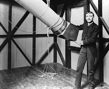
On this date 140 years ago, American physician and prominent amateur astronomer Henry Draper (1837-1882) made the first successful photograph of the Great Nebula in Orion, now usually referred to as the Orion Nebula. He used an 11-inch telescope (an Alvan Clark refractor!) and an exposure time of 50 minutes for the black and white photograph.
First photograph of the Orion Nebula, September 30, 1880. (Henry Draper)
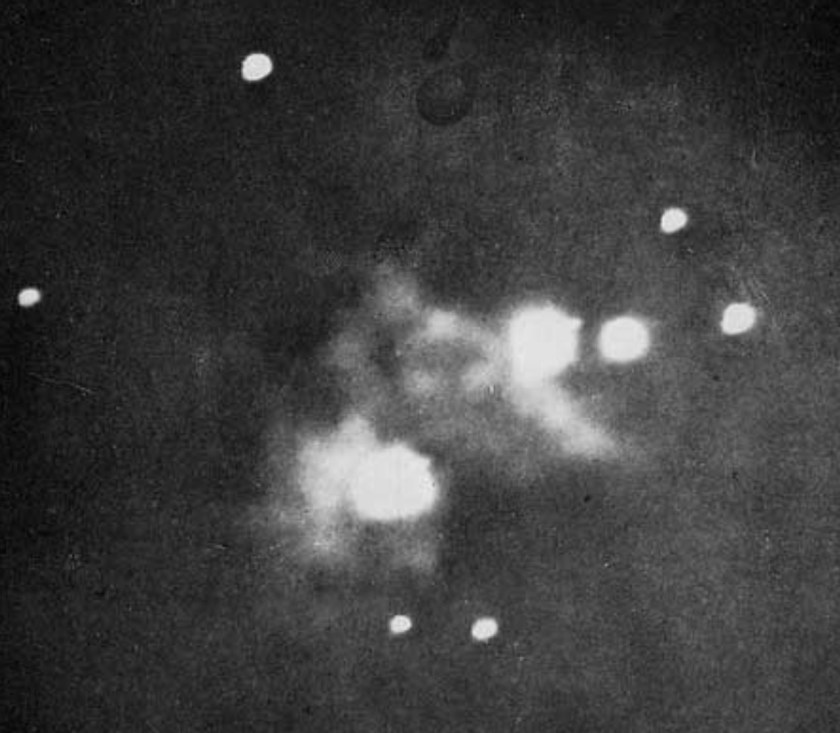
Draper continued to improve his technique, and a year and a half later he obtained a 137-minute exposure showing much more detail.
Photograph of the Orion Nebula, March 14, 1882. (Henry Draper)
It really is amazing how image recording technology has improved over the past century and a half! At its best, film-based photography had a quantum efficiency of only about 2%, which means that only 2 out of every 100 photons of light impinging on the photographic medium is actually recorded. The rest is reflected or absorbed. The human eye—when well dark adapted—has a quantum efficiency of 15% or better, easily besting photography. Why, then, do photographs of deep sky objects show so much more detail than what can be seen through the eyepiece? The explanation is that the human eye can integrate photons and hold an image for only about 0.1 second. Film, on the other hand, can hold an image much longer. Even with reciprocity failure, photographic media like film can collect photons for minutes or even hours, giving them a big advantage over the human eye. But charge-coupled devices (CCDs) are a considerable improvement over older technologies since they typically have a quantum efficiency of 70% up to 90% or more. The CCD has truly revolutionized both professional and amateur astronomy in recent decades.
I attended the 234th meeting of the American Astronomical Society (AAS), held in St. Louis, Missouri, June 9-13, 2019. Here are some highlights from that meeting.
Day 1 – Monday, June 10, 2019
Research Notes of the AAS is a non-peer-reviewed, indexed and secure record of works in progress, comments and clarifications, null results, or timely reports of observations in astronomy and astrophysics. RNAAS.
The Bulletin of the American Astronomical Society is the publication for science meeting abstracts, obituaries, commentary articles about the discipline, and white papers of broad interest to our community. BAAS.
We still have many unanswered questions about galaxy formation. The rate of star formation in galaxies and central black hole accretion activity was highest between 10 and 11 billion years ago. This corresponds to redshift z around 2 to 3, referred to as “cosmic high noon”. This is the ideal epoch for us to answer our questions about galaxy formation. Near-infrared spectroscopy is important to the study of galaxies during this epoch, and we are quite limited in what we can do from terrestrial observatories. Space based telescopes are needed, and the James Webb Space Telescope (JWST) will be key.
Galaxies are not closed boxes. We need to understand how inflows and outflows affect their evolution (“galactic metabolism”).
There are five international space treaties, with the Outer Space Treaty of 1967 being the first and most important. The United States has signed four of the five treaties. The Moon Agreement of 1979 which states that no entity can own any part of the Moon does not include the United States as one of the signatories.
U.S. Code 51303, adopted in 2015, identifies asteroid resource and space resource rights, and states that “A United States citizen engaged in commercial recovery of an asteroid resource or a space resource under this chapter shall be entitled to any asteroid resource or space resource obtained, including to possess, own, transport, use, and sell the asteroid resource or space resource obtained in accordance with applicable law, including the international obligations of the United States.”
So, unfortunately, U.S. law does allow a commercial entity to own an asteroid, but you have to get there first before you can claim it. The large metallic asteroid 16 Psyche is highly valuable and will probably be owned by some corporation in the not-too-distant future.
Space law often relies upon maritime law as a model.
Astronomer Vayu Gokhale from Truman State University gave an interesting iPoster Plus presentation on how he and his students are operating three automated and continuous zenithal sky brightness measurement stations using narrow-field Sky Quality Meters (SQMs) from Unihedron. Even measurements when it is cloudy are of value, as clouds reflect light pollution back towards the ground. Adding cloud type and height would allow us to make better use of cloudy-night sky brightness measurements. In a light-polluted area, the darkest place is the zenith, and clouds make the sky brighter. In an un-light-polluted area, the darkest place is the horizon, and clouds make the sky darker.
A number of precision radial velocity instruments for exoplanet discovery and characterization will begin operations soon or are already in operation: NEID, HARPS, ESPRESSO, EXPRES, and iLocater, to name a few.
Dark matter: clumps together under gravity, does not emit, reflect, or absorb electromagnetic radiation, and does not interact with normal matter in any way that causes the normal matter to emit, reflect, or absorb electromagnetic radiation. The ratio between dark matter and normal (baryonic matter) in our universe is 5.36 ± 0.05 (Planck 2018).
What is dark matter? It could be a new particle. If so, can we detect its non-gravitational interactions? It could be macroscopic objects, perhaps primordial black holes. Or, it could be a mixture of both. Another possibility is that a modification to the laws of gravitation will be needed to mimic the effects of dark matter.
How “dark” is dark matter? Does it interact at all (besides gravitationally)? Can dark matter annihilate or decay? Even if dark matter started hot, it cools down rapidly as the universe expands.
Primordial black holes could have masses ranging anywhere between 10-16 and 1010 solar masses. LIGO is possibility sensitive to colliding primordial black holes with masses in the range of a few to a few hundred solar masses. Primordial black holes are a fascinating dark matter candidate, with broad phenomenology.
The Cosmic Microwave Background (CMB) is a nearly perfect blackbody with distortions < 1 part in 10,000. What this tells us is that nothing dramatically heated or cooled photons after 2 months after the Big Bang. Anisotropies are variances in the CMB temperature, and the angular power spectrum is variance of CMB temperature as a function of angular scale. CMB anisotropies are very sensitive to the ionization history of the universe. How the universe recombined plays a key role in CMB anisotropies.
Hydrogen: not such a simple atom.
The CMB is polarized. The polarization is caused by Mie scattering of photons.
At the NASA Town Hall, we learned about current and future missions: TESS, SPHEREx, HabEx, LUVOIR, Lynx, Origins Space Telescope (OST).
The highest image rate of standard CCD and CMOS video cameras for asteroid occultation work is 30 frames (60 fields) per second, providing time resolution of 0.017 seconds per field. Adaptive optics and autoguider imaging devices often have a higher sampling rate, and such a camera could perhaps be easily modified to be used for occultation work. A time-inserter would need to be added to the camera (either on-board or GPS-based), and improvements in quantum efficiency (because of the shorter exposures) would benefit from newer imaging technologies such as a Geiger-mode avalanche photodiode (APD); or the Single-photon avalanche detector (SPAD), which are frequently used in chemistry.
Gregory Simonian, graduate student at Ohio State, presented “Double Trouble: Biases Caused by Binaries in Large Stellar Rotation datasets”. The Kepler data yielded 34,030 rotation periods through starspot variability. However, the rapid rotators are mostly binaries. In the Kepler dataset, many rapid rotators have a spin period of the stars equal to the orbital period of the binary. These eclipsing binaries, also known as photometric binaries because they are detected through changes in brightness during eclipses and transits, need to be treated separately in stellar rotation datasets.
Granulation was discovered by William Herschel in 1801 and are vertical flows in the solar photosphere on the order of 1000 m/s, and 1000 km horizontal scale. Supergranulation (Hart 1954, Leighton et al. 1962) are horizontal motions in the photosphere of 300 to 500 m/s with a horizontal scale on the order of 30,000 km.
The amplitude of oscillations in red giants increase dramatically with age.
We’ve never observed the helium flash event in a red giant star, though models predict that it must occur. It is very brief and would be difficult to detect observationally.
Brad Schaefer, Professor Emeritus at Louisiana State University, gave a talk on “Predictions for Upcoming Recurrent Nova Eruptions”. Typically, recurrent novae have about a 30% variation in eruptive timescales, so predicting the next eruption is not trivial. Due to the solar gap (when the object is too close to the Sun to observe on or near the Earth), we are obviously missing some eruptions. However, orbital period changes (O-C curve) can tell us about an eruption we missed. U Sco and T CrB are well-known examples of recurrent novae. Better monitoring of recurrent novae is needed during the pre-eruption plateau. Monitoring in the blue band is important for prediction.
I had the good fortune to talk with Brad on several occasions during the conference, and found him to be enthusiastic, knowledgeable, and engaging. Perhaps you have seen The Remarkable Science of Ancient Astronomy (The Great Courses), and he is just as articulate and energetic in real life. Among other things, we discussed how the internet is filled with misinformation, and even after an idea has been convincingly debunked, the misinformation continues to survive and multiply in cyberspace. This is a huge problem in the field of archaeoastronomy and, indeed, all fields of study. People tend to believe what they want to believe, never mind the facts.
Astrobites is a daily astrophysical-literature blog written by graduate students in astronomy around the world. The goal of Astrobites is to present one interesting paper from astro-ph per day in a brief format accessible to its target audience: undergraduate students in the physical sciences who are interested in active research.
Helioseismology can be done both from space (all) and the ground (some). Active regions on the far side of the Sun can be detected with helioseismology.
All HMI (Helioseismic and Magnetic Imager) data from the Solar Dynamics Observatory is available online.
A good approach to studying solar data is to subtract the average differential rotation at each point/region on the Sun and look at the residuals.
The Wilcox Solar Observatory has been making sun-as-a-star mean magnetic field measurements since 1975.
It is possible to infer electric currents on the Sun, but this is much more difficult than measuring magnetic fields.
Future directions in solar studies: moving from zonal averages to localized regions in our modeling, and the ability through future space missions to continuously monitor the entire surface of the Sun at every moment.
Systematic errors are nearly always larger than statistical uncertainty.
Day 2 – Tuesday, June 11, 2019
It is probably not hyperbole to state that every star in our galaxy has planets. About 1/5 of G-type stars have terrestrial planets within the habitable zone. Life is widespread throughout the universe.
Gas-grain interaction is at the core of interstellar chemistry. Interstellar ices, charged ices, surface chemistry – there is more time for interactions to occur on a dust grain than in a gas. Grain collisions are important, too.
Hot cores are transient regions surrounding massive protostars very early in their evolution. Similar regions are identified around low-mass protostars and are called corinos.
Methanol (CH3OH) is key to making simple organic molecules (SOM). Evaporating ice molecules drive rich chemistry. Dust plays a key role in the chemistry and in transporting material from the interstellar medium (ISM) to planetary systems.
The Rosetta mission detected amino acids on comet 67P/Churyumov–Gerasimenko.
JUICE (JUpiter ICy moons Explorer) is an ESA mission scheduled to launch in 2022, will enter orbit around Jupiter in October 2029 and Ganymede in 2032. It will study Europa, Ganymede, and Callisto in great detail.
The gravitational wave event GW170817 (two infalling and colliding neutron stars) was also detected as a gamma-ray burst (GRB) by the Fermi gamma-ray space telescope, which has a gamma-ray burst detector that at all times monitors the 60% of the sky that is not blocked by the Earth.
The time interval between the GW and GRB can range between tens of milliseconds up to 10 seconds.
The Milky Way galaxy circumnuclear disk is best seen at infrared wavelengths around 50 microns. Linear polarization tells us the direction of rotation. The star cluster near the MW center energizes and illuminates gas structures. Gravity dominates in this region. The role of magnetic fields in this region has been a mystery.
Pitch angle – how tightly wound the spiral arms are in a spiral galaxy.
Are spiral arms transient or long lived? They are probably long lived. There may be different mechanisms of spiral arm formation in grand design spirals compared with other types of spiral galaxies.
In studying spiral galaxies, we often deproject to face-on orientation.
The co-rotation radius is the distance from the center of a spiral galaxy beyond which the stars orbit slower than the spiral arms. Inside this radius, the stars move faster than the spiral arms.
The Sun is located near the corotation circle of the Milky Way.
The origins of supermassive black holes (SMBH) at the centers of galaxies are unclear. Were they seeded from large gas clouds, or were they built up from smaller black holes?
The black holes at the centers of spiral galaxies tend to be more massive when the spiral arm winding is tight, and less massive when the spiral arm winding is loose.
Spiral Graph is in review as a Zooniverse project and has not yet launched. Citizen scientists will trace the spiral arms of 6,000 deprojected spiral galaxies, and 15 traces will be needed for each galaxy. Spiral arm tracings will provide astronomers with intermediate mass black hole candidate galaxies.
Barred spiral galaxies are very common. 66% to 75% of spiral galaxies show evidence of a bar at near-infrared wavelengths.
Magnetic fields in the inner regions of spiral galaxies are scrambling radio emissions to some extent, but radio astronomers have ways to deal with this.
For me, the plenary lecture given by Suvrath Mahadevan, Pennsylvania State University, was the first truly outstanding presentation. His topic was “The Tools of Precision Measurement in Exoplanet Discovery: Peeking Under the Hood of the Instruments”. His discussion of the advance in radial velocity instrumentation was revelatory to me, as his starting point was Roger F. Griffin’s radial velocity spectrometer we used at Iowa State University in the 1970s and 1980s, giving us a precision of about 1 km/s. My, we have come a long way since then!
To discover our Earth from another star system in the ecliptic plane would require detecting an 8.9 cm/s velocity shift in the Sun’s motion over the course of a year.
Precision radial velocity measurement requires we look at the displacement of thousands of spectral lines using high resolution spectroscopy.
The two main techniques are 1) Simultaneous reference and 2) Self reference (iodine cell). Also, externally dispersed interferometry and heterodyne spectroscopy can be used.
Griffin 1967 ~ km/s → CORAVEL 1979 ~300 m/s → CORALIE/ELODIE 1990 ~ 5-10 m/s → HARPS 2000 ~ 1 m/s → ESPRESSO/VLT, EXPRES/DCT, NEID/KPNO, HPF/HET.
We cannot build instruments that are stable over time at 10 cm/s resolution or less.
You can track the relative change in velocity much better than absolute velocity because of the “noise” generated by stellar internal motions.
Measuring the radial velocity at red or infrared wavelengths is best for M dwarfs, and cooler stars.
High radial velocity precision will require long-term observations, and a better understanding of and mitigation for stellar activity. Many things need to be considered: telescope, atmosphere, barycentric correction (chromatic effects can lead to 1/2 m/s error), fibers, modal noise, instrument decoupled from the telescope, calibrators, optics, stability, pipeline, etc. Interdisciplinary expertise is required.
NEID will measure wavelengths of 380 – 930 nm, and have a spectral resolution of R ~ 90,000.
Pushing towards 10 cm/s requires sub-milli-Kelvin instrument stability high-quality vacuum chambers, octagonal fibers, scrambling, and excellent guiding of the stellar image on the fiber to better than 0.05 arcseconds.
Precision radial velocity instruments such as NEID and HPF weigh two tons, so at present they can only be used with ground-based telescopes.
Charge Transfer Efficiency (CTE): need CCDs with CTE > 0.999999. Other CCD issues that don’t flat field out accurately: CCD stitch boundaries, cross hatching in NIR detectors, crystalline defects, sub-pixel quantum efficiency differences. Even the act of reading out the detector introduces a noise source.
10 cm/s is within reach from a purely instrumental perspective, but almost everything has to be just right. But we need to understand stellar activity better: granulation, supergranulation, flares, oscillations, etc. We may not be able to isolate these components of stellar activity, but we will certainly learn a lot in the process.
1s time resolution is required to properly apply barycentric corrections.
Andrew Fraknoi gave an update on the OpenStax Astronomy text.
about 70 people have been involved in its development and vetting
each chapter includes collaborative group activities
math examples are in separate boxes
it is estimated that 500+ institutions have adopted this online and free introductory astronomy textbook, and ~200,000 students have used it, including ~30,000 amateur astronomers
multiple choice question bank for registered instructors
The surface of the Moon has a thinner atmosphere than low-Earth orbit.
Kenneth Gayley, University of Iowa, gave an interesting short talk, “The Real Explanation for Type Ia Supernovae and the Helium Flash”. Here’s the abstract: https://ui.adsabs.harvard.edu/abs/2019AAS…23422404G/abstract . I’m looking forward to reading the entire paper.
Gene Byrd, University of Alabama, gave an interesting short presentation, “Two Astronomy Demos”. The first was “Stars Like Grains of Sugar”, reminiscent of Archimedes’ The Sand Reckoner. And “Phases with the Sun, Moon, and Ball”. He uses a push pin in a golf ball (the golf ball even has craters!). Morning works best for this activity. The Sun lights the golf ball and the Moon and they have the same phase—nice! Touching as well as seeing the golf ball helps students understand the phases of the Moon. Here’s a link to his paper on these two activities.
Daniel Kennefick, University of Arkansas, gave a short presentation on the 1919 eclipse expedition that provided experimental evidence (besides the correct magnitude of the perihelion precession of Mercury) that validated Einstein’s General Relativity. Stephen Hawking in his famous book A Brief History of Time mis-remembered that the 1979 re-analysis of the Eddington’s 1919 eclipse data showed that he may “fudged” the results to prove General Relativity to be correct. He did not! See Daniel Kennefick’s new book on the subject, No Shadow of a Doubt: The 1919 Eclipse That Confirmed Einstein’s Theory of Relativity.
Brad Schaefer, Louisiana State University, gave another engaging talk, presenting evidence that the Australian aborigines may have discovered the variability of the star Betelgeuse, much earlier than the oft-stated discovery by John Herschel in 1836. Betelgeuse varies in brightness between magnitude 0.0 and +1.3 quasi-periodically over a period of about 423 days. It has been shown that laypeople can detect differences in brightness as small as 0.3 magnitude with the unaided eye, and with good comparison stars (like Capella, Rigel, Procyon, Pollux, Adhara, and Bellatrix—not all of which are visible from Australia—for Betelgeuse). It is plausible that the variability of Betelgeuse may have been discovered by many peoples at many different times. The Australian aborigines passed an oral tradition through many generations that described the variability of Betelgeuse. https://ui.adsabs.harvard.edu/abs/2019AAS…23422407S/abstract.
As a longtime astronomical observer myself, I have actually never noticed the variability of Betelgeuse, but Brad has. After his presentation, I mentioned to Brad that it would be interesting to speculate what would lead early peoples to look for variability in stars in the first place, which seems to me to be a prerequisite for anyone discovering the variability of Betelgeuse. His response pointed out that all it would take is one observant individual in any society who would notice/record the variability and then point it out to others.
During the last plenary session of the day, it was announced that the Large Synoptic Survey Telescope (LSST), which is expected to see first light in 2020, is expected to be renamed the Vera Rubin Survey Telescope. Tremendous applause followed! https://aas.org/posts/news/2019/06/lsst-may-be-renamed-vera-rubin-survey-telescope .
If you haven’t looked at the NASA/IPAC Extragalactic Database (NED) lately, you will find new content and functionality. It has been expanded a great deal, and now includes many stellar objects, because we don’t always know what is really a star and what is not. There is now a single input field where you can enter names, coordinates with search radius, etc. NED is “Google for Galaxies”.
I noticed during the 10-minute iPoster Plus sessions that there is a countdown timer displayed unobtrusively in the upper right hand corner that helps the presenter know how much time they have remaining. I think this would be a great device for anyone giving a short presentation in any venue.
Day 3 began with what for me was the finest presentation of the entire conference: Joshua Winn, Princeton University, speaking on “Transiting Exoplanets: Past, Present, and Future”. I first became familiar with Josh Winn through watching his outstanding video course, The Search for Exoplanets: What Astronomers Know, from The Great Courses. I am currently watching his second course, Introduction to Astrophysics, also from The Great Courses. Josh is an excellent teacher, public speaker, and presenter, and it was a great pleasure to meet him at this conference.
Transits provide the richest source of information we have about exoplanets. For example, we can measure the obliquity of the star’s equator relative to the planet’s orbital plane by measuring the apparent Doppler shift of the star’s light throughout transit.
Who was the first to observe a planetary transit? Pierre Gassendi (1592-1655) was the first to observe a transit of Mercury across the Sun in November 1631. Jeremiah Horrocks (1618-1641) was the first to observe a transit of Venus across the Sun in November 1639. Christoph Scheiner (1573-1650) claimed in January 1612 that spots seen moving across the Sun were planets inside Mercury’s orbit transiting the Sun, but we know know of course that sunspots are magnetically cooled regions in the Sun’s photosphere and not orbiting objects at all. Though Scheiner was wrong about the nature of sunspots, his careful observations of them led him to become the first to measure the Sun’s equatorial rotation rate, the first to notice that the Sun rotated more slowly at higher latitudes, and the first to notice that the Sun’s equator is tilted with respect to the ecliptic, and to measure its inclination.
An exoplanet can be seen to transit its host star if the exoplanet’s orbit lies within the transit cone, an angle of 2R*/a centered on our line of sight to the star. R* is the star’s radius, and a is the semi-major axis of the planet’s orbit around the star.
Because of the geometry, we are only able to see transits of 1 out of every 215 Earth-Sun analogs.
Space is by far the best place to study transiting exoplanets.
If an exoplanet crosses a starspot, or a bright spot, on the star, you will see a “blip” in the transit light curve that looks like this:
Transiting exoplanet crossing a starspot (left) or bright spot (right) in the photosphere of the star
Are solar systems like our own rare? Not at all! There are powerful selection effects at work in exoplanet transit statistics. We have discovered a lot of “hot Jupiters” because large, close-in planets are much easier to detect with their short orbital periods and larger transit cones. In actuality, only 1 out of every 200 sun-like stars have hot Jupiters.
Planet statistical properties was the main goal of the Kepler mission. Here are some noteworthy discoveries:
Kepler 89 – two planets transiting at the same time (only known example)
Kepler 36 – chaotic three-body system
Kepler 16 – first known transiting exoplanet in a circumbinary orbit
Transiting Exoplanet Survey Satellite (TESS) – Unlike Kepler, which is in an Earth-trailing heliocentric orbit, TESS is in a highly-elliptical orbit around the Earth with an apogee approximately at the distance of the Moon and a perigee of 108,000 km. TESS orbits the Earth twice during the time the Moon orbits once, a 2:1 orbital resonance with the Moon.
TESS has four 10.5 cm (4-inch) telescopes, each with a 24˚ field of view. Each TESS telescope is constantly monitoring 2300 square degrees of sky.
TESS is fundamentally about short period planets. Data is posted publicly as soon as it is calibrated. TESS has already discovered 700 planet candidates. About 1/2 to 2/3 will be true exoplanets. On average, TESS is observing stars that are about 4 magnitudes brighter than stars observed by Kepler.
The TESS Follow-Up Observing Program (TFOP) is a large working group of astronomical observers brought together to provide follow-up observations to support the TESS Mission’s primary goal of measuring the masses for 50 planets smaller than 4 Earth radii, in addition to organizing and carrying out follow-up of TESS Objects of Interest (TOIs).
HD 21749 – we already had radial velocity data going back several years for this star that hosts an exoplanet that TESS discovered
Gliese 357 – the second closest transiting exoplanet around an M dwarf, after HD 219134
TESS will tell us more about planetary systems around early-type stars.
TESS will discover other transient events, such as supernovae, novae, variable stars, etc. TESS will also make asteroseismology measurements and make photometric measurements of asteroids.
The James Webb Space Telescope (JWST) will be able to do follow-up spectroscopy of planetary atmospheres.
Upcoming exoplanet space missions: CHEOPS, PLATO, and WFIRST.
Hot Jupiter orbits should often be decaying, so this is an important area of study.
Sonification is the process of turning data into sound. For example, you could “listen” to a light curve (with harmonics, e.g. helioseismology and asteroseismology) of a year’s worth a data in just a minute or so.
Solar cycles have different lengths (11-ish years…).
Some predictions: 2019 will be the warmest year on record, 2020 will be less hot. Solar cycle 24 terminate in April 2020. Solar cycle 25 will be weaker than cycle 24. Cycle 25 will start in 2020 and will be the weakest in 300 years, the maximum (such as it is) occurring in 2025. Another informed opinion was that Cycle 25 will be comparable to Cycle 24.
Maunder minimum: 1645 – 1715
Dalton minimum: 1790 – 1820
We are currently in the midst of a modern Gleissberg minimum. It remains to be seen if it will be like the Dalton minimum or a longer “grand minimum” like the Maunder minimum.
Citizen scientists scanning Spitzer Space Telescope images in the Zooniverse Milky Way Project, have discovered over 6,000 “yellow balls”. The round features are not actually yellow, they just appear that way in the infrared Spitzer image color mapping.
Yellow balls (YBs) are sites of 8 solar mass or more star formation, surrounded by ionized hydrogen (H II) gas. YBs thus reveal massive young stars and their birth clouds.
Antlia 2 is a low-surface-brightness (“dark”) dwarf galaxy that crashed into our Milky Way galaxy. Evidence for this collision comes from “galactoseismology” which is the study of ripples in the Milky Way’s disk.
The Large Magellanic Cloud (LMC), Small Magellanic Cloud (SMC), and the Sagittarius Dwarf Galaxy have all affected our Milky Way Galaxy, but galactoseismology has shown that there must be another perturber that has affected the Milky Way. Antlia 2, discovered in November 2018 from data collected by the Gaia spacecraft, appears to be that perturber.
Gaia Data Release 2 (DR2) indicates that the Antlia 2 dwarf galaxy is about 420,000 ly distant, and it is similar in extent to the LMC. It is an ultra-diffuse “giant” dwarf galaxy whose stars average two magnitudes fainter than the LMC. Antlia 2 is located 11˚ from the galactic plane and has a mass around 1010 solar masses.
A question that is outstanding is what is the density of dark matter in Antlia 2? In the future, Antlia 2 may well be an excellent place to probe the nature of dark matter.
Gravity drives the formation of cosmic structure, dark energy slows it down.
Stars are “noise” for observational cosmologists.
“Precision” cosmology needs accuracy also.
The Vera Rubin telescope (Large Synoptic Survey Telescope) in Chile will begin full operations in 2022, collecting 20 TB of data each night!
We have a “galaxy bias” – we need to learn much more about the relation between galaxy populations and matter distribution.
Might there be an irregular asymmetric cycle underlying the regular 22-year sunspot cycle? The dominant period associated with this asymmetry is around 35 to 50 years.
The relationship between differential rotation and constant effective temperature of the Sun: the Sun has strong differential rotation along radial lines, and there is little variation of solar intensity with latitude.
Solar filaments (solar prominences) lie between positive and negative magnetic polarity regions.
Alfvén’s theorem: in a fluid with infinite electric conductivity, the magnetic field is frozen into the fluid and has to move along with it.
Some additional solar terms and concepts to look up and study: field line helicity, filament channels, kinetic energy equation, Lorentz force, magnetic energy equation, magnetic flux, magnetic helicity, magnetohydrodynamics (MHD), meridional flow, polarity inversion lines, relative helicity, sheared arcade, solar dynamo.
We would like to be able to predict solar eruptions before they happen.
Magnetic helicity is injected by surface motions.
It accumulates at polarity inversion lines.
It is removed by coronal mass ejections.
Day 4 – Thursday, June 13, 2019
Cahokia (our name for it today) was the largest city north of Mexico 1,000 years ago. It was located at the confluence of the Mississippi, Missouri, and Illinois Rivers. At its height from 1050 – 1200 A.D., Cahokia city covered 6 square miles and had 10,000 to 20,000 people. Cahokia was a walled city. Some lived inside the walls, and others lived outside the walls.
Around 120 mounds were built at greater Cahokia; 70 are currently protected. Platform mounds had buildings on top, and some mounds were used for burial and other uses.
Monks mound is the largest prehistoric earthwork in the Americas. Mound 72 has an appalling history.
Woodhenge – controversial claim that it had an astronomical purpose. Look up Brad Schaefer’s discussion, “Case studies of three of the most famous claimed archaeoastronomical alignments in North America”.
Cahokia’s demise was probably caused by many factors, including depletion of resources and prolonged drought. We do not know who the descendents of the Cahokia people are. It is possible that they died out completely.
The Greeks borrowed many constellations from the Babylonians.
One Sky, Many Astronomies
The neutron skin of a lead nucleus (208Pb) is a useful miniature analog for a neutron star.
Infalling binary neutron stars, such as GW 170817, undergo tidal deformation.
SmallSats
Minisatellite: 100-180 kg
Microsatellite: 10-100 kg
Nanosatellite: 1-10 kg
Picosatellite: 0.01-1 kg
Femtosatellite: 0.001-0.01 kg
CubeSats are a class of nanosatellites that use a standard size and form factor. The standard CubeSat size uses a “one unit” or “1U” measuring 10 × 10 × 10 cm and is extendable to larger sizes, e.g. 1.5, 2, 3, 6, and even 12U.
The final plenary lecture and the final session of the conference was a truly outstanding presentation by James W. Head III, Brown University, “The Apollo Lunar Exploration Program: Scientific Impact and the Road Ahead”. Head is a geologist who trained the Apollo astronauts for their Moon missions between 1969 and 1972.
During the early years of the space program, the United States was behind the Soviet Union in space technology and accomplishments. The N1 rocket was even going to deliver one or two Soviet cosmonauts to lunar orbit so they could land on the Moon.
Early in his presidency, John F. Kennedy attempted to engage the Soviet Union in space cooperation.
Chris Kraft’s book, Flight: My Life in Mission Control is recommended.
The Apollo astronauts (test pilots) were highly motivated students.
The United States flew 21 robotic precursor missions to the Moon in the eight years before Apollo 11. Rangers 1-9 were the first attempts, but 1 through 6 were failures and we couldn’t even hit the Moon.
Head recommends the recent documentary, Apollo 11, but called First Man Hollywood fiction, saying, “That is not the Neil Armstrong I knew.”
The Apollo 11 lunar samples showed us that the lunar maria (Mare Tranquillitatis) has an age of 3.7 Gyr and has a high titanium abundance.
The Apollo 12 lunar excursion module (LEM) landed about 600 ft. from the Surveyor 3 probe in Oceanus Procellarum, and samples from that mission were used to determine the age of that lunar maria as 3.2 Gyr.
Scientists worked shoulder to shoulder with the engineers during the Apollo program, contributing greatly to its success.
Apollo 11 landed at lunar latitude 0.6˚N, Apollo 12 at 3.0˚S, Apollo 14 at 3.6˚S, and Apollo 15 at 26.1˚N. Higher latitude landings required a plane change and a more complex operation to return the LEM to the Command Module.
The lunar rover was first used on Apollo 15, and allowed the astronauts to travel up to 7 km from the LEM. Head said that Dave Scott did remarkable geological investigations on this mission. He discovered and returned green glass samples, and in 2011 it was determined that there is water inside those beads. Scott also told a little fib to Mission Control to buy him enough time to pick up a rock that turned out to be very important, the “seat belt basalt”.
In speaking about Apollo 16, Head called John Young “one of the smartest astronauts in the Apollo program”.
Harrison Schmitt, Apollo 17, was the only professional geologist to go to the Moon, and he discovered the famous “orange soil”. This is the mission where the astronauts repaired a damaged fender on the lunar rover using duct tape and geological maps to keep them from getting covered in dust while traveling in the rover.
When asked about the newly discovered large mass under the lunar surface, Head replied that it is probably uplifted mantle material rather than an impactor mass underneath the surface.
Radiometric dating of the Apollo lunar samples have errors of about ± 5%.
One of the reasons the Moon’s albedo is low is that space weather has darkened the surface.
The South Pole-Aitken basin is a key landing site for future exploration. In general, both polar regions are of great interest.
Smaller objects like the Moon and Mars cooled efficiently after their formation because of their high surface area to volume ratio.
We do not yet know if early Mars was warm and wet, or cold and icy with warming episodes. The latter is more likely if our solar system had a faint young sun.
Venus has been resurfaced in the past 0.5 Gyr, and there is no evidence of plate tectonics. The first ~80% of the history of Venus is unknown. Venus probably had an ocean and tectonic activity early on, perhaps even plate tectonics. Venus may have undergone a density inversion which exchanged massive amounts of material between the crust and mantle. 80% of the surface of Venus today is covered by lava flows.
A mention was made that a new journal of Planetary Science (in addition to Icarus, presumably) will be coming from the AAS soon.
I attend a lot of meetings and lectures (both for astronomy and SAS), and I find that I am one of the few people in attendance who write down any notes. Granted, a few are typing at their devices, but one never knows if they are multitasking instead. For those that don’t take any notes, I wonder, how do they really remember much of what they heard days or weeks later without having written down a few keywords and phrases and then reviewing them soon after? I did see a writer from Astronomy Magazine at one of the press conferences writing notes in a notebook as I do. I believe it was Jake Parks.
Anyone who knows me very well knows that I love traveling by train. To attend the AAS meeting, I took a Van Galder bus from Madison to Chicago, and then Amtrak from Chicago to St. Louis. Pretty convenient that the AAS meeting was held at the Union Station Hotel, just a few blocks from Amtrak’s Gateway Station. It is a fine hotel with a lot of history, and has an excellent on-site restaurant. I highly recommend this hotel as a place to stay and as a conference venue.
The bus and train ride to and fro afforded me a great opportunity to catch up on some reading. Here are a few things worth sharing.
astrometry.net – you can upload your astronomical image and get back an image with all the objects in the image astrometrically annotated. Wow!
16 Psyche, the most massive metal-rich asteroid, is the destination for a NASA orbiter mission that is scheduled to launch in 2022 and arrive at Psyche in 2026. See my note about 16 Psyche in the AAS notes above.
The lowest hourly meteor rate for the northern hemisphere occurs at the end of March right after the vernal equinox.
A tremendous, dynamic web-based lunar map is the Lunar Reconnaissance Orbiter Camera (LROC) Quickmap, quickmap.lroc.asu.edu.
I read with great interest Dr. Ken Wishaw’s article on pp. 34-38 in the July 2019 issue of Sky & Telescope, “Red Light Field Test”. Orange or amber light is probably better that red light for seeing well in the dark while preserving your night vision. You can read his full report here. Also, see my article “Yellow LED Astronomy Flashlights” here.
Jupiter and Saturn will have a spectacular conjunction next year. As evening twilight fades on Monday, December 21, 2020, the two planets will be just 1/10th of a degree apart, low in the southwestern sky.
An oblate spheroid with axes a = b > c is called a Maclaurin spheroid. If all three axes have different lengths a > b > c, then you have a Jacobi ellipsoid.
The light curve of a stellar occultation by a minor planet (asteroid or TNO) resembles a square well if the object has no atmosphere (or one so thin that it cannot be detected, given the sampling rate and S/N), and the effects of Fresnel diffraction and the star’s angular diameter are negligible.
Astronomer Margaret Burbidge, who turns 100 on August 12, 2019, refused the AAS Annie Jump Cannon Award in 1972, stating in her rejection letter that “it is high time that discrimination in favor of, as well as against, women in professional life be removed, and a prize restricted to women is in this category.” In 1976, Margaret Burbidge became the first woman president of the AAS, and in 1978 she announced that the AAS would no longer hold meetings in the states that had not ratified the Equal Rights Amendment (ERA).
During the days following the conference when I was writing this report, I received the happy news from both the AAS and Sky & Telescope that AAS was the winning bidder of S&T during a bankruptcy auction of its parent company, F+W Media. I believe that this partnership between the AAS and Sky & Telescope will benefit both AAS members and S&T readers immensely. Peter Tyson, Editor in Chief of Sky & Telescope, stated in the mutual press release, “It feels like S&T is finally landing where it belongs.” I couldn’t agree more!
Planetary orbits are randomly oriented throughout our galaxy. The probability that an exoplanet’s orbit will be fortuitously aligned to allow that exoplanet to transit across the face of its parent star depends upon the radius of the star, the radius of the planet, and the distance of the planet from the star. In general, planets orbiting close-in are more likely to be seen transiting their star then planets orbiting further out.
The equation for the probability of observing a exoplanet transit event is
where ptra is the transit probability, R* is the radius of the star, Rp is the radius of the planet, a is the semi-major axis of the planetary orbit, and e is the eccentricity of the planetary orbit
Utilizing the data in the NASA Exoplanet Archive for the 1,463 confirmed exoplanets where the above data is available (and assuming e = 0 when eccentricity is unavailable), we find that the median exoplanet transit probability is 0.0542. This means that, on average, 1 out of every 18 planetary systems will be favorably aligned to allow us to observe transits. However, keep in mind that our present sample of exoplanets is heavily biased towards large exoplanets orbiting close to their parent star. Considering a hypothetical sample of Earth-sized planets orbiting 1 AU from a Sun-sized star, the transit probability drops to 0.00469, which means that we would be able to detect only about 1 out of every 213 Earth-Sun analogs using the transit method.
How might we detect some of the other 99.5%? My admired colleague in England, Abdul Ahad, has written a paper about his intriguing idea: “Detecting Habitable Exoplanets During Asteroidal Occultations”. Abdul’s idea in a nutshell is to image the immediate environment around nearby stars while they are being occulted by asteroids or trans-Neptunian objects (TNOs) in order to detect planets orbiting around them. While there are many challenges (infrequency of observable events, narrow shadow path on the Earth’s surface, necessarily short exposure times, and extremely faint planetary magnitudes), I believe that his idea has merit and will one day soon be used to discover and characterize exoplanets orbiting nearby stars.
Ahad notes that the apparent visual magnitude of any given exoplanet will be directly proportional to the apparent visual magnitude of its parent star, since exoplanets shine by reflected light. Not only that, Earth-sized and Earth-like planets orbiting in the habitable zone of any star would shine by reflected light of the same intrinsic brightness, regardless of the brightness of the parent star. He also notes that the nearer the star is to us, the greater will be a given exoplanet’s angular distance from the occulted star. Thus, given both of these considerations (bright parent star + nearby parent star = increased likelihood of detection), nearby bright stars such as Alpha Centauri A & B, Sirius A, Procyon A, Altair, Vega, and Fomalhaut offer the best chance of exoplanet detection using this technique.
Since an exoplanet will be easiest to detect when it is at its greatest angular distance from its parent star, we will be seeing only about 50% of its total reflected light. An Earth analog orbiting Alpha Centauri A would thus shine at visual magnitude +23.7 at 0.94″ angular distance, and for Alpha Centauri B the values would be +24.9 and 0.55″.
Other considerations include the advantage of an extremely faint occulting solar system object (making it easier to detect faint exoplanets during the occultation event), and the signal boost offered by observing in the infrared, since exoplanets will be brightest at these wavelengths.
A distant (and therefore slow-moving) TNO would be ideal, but the angular size of the TNO needs to be larger than the angular size of the occulted star. However, slow-moving objects mean that occultation events will be rare.
The best chance of making this a usable technique for exoplanet discovery would be a space-based observatory that could be positioned at the center of the predicted shadow and would be able to move along with the shadow to increase exposure times (Ahad, personal communication). It would be an interesting challenge in orbital mechanics to design the optimal base orbit for such a spacecraft. The spacecraft orbit would be adjusted to match the position and velocity of the occultation shadow for each event using an ion drive or some other electric propulsion system.
One final thought on the imaging necessary to detect exoplanets using this technique. With a traditional CCD you would need to begin and end the exoplanet imaging exposure(s) only while the parent star is being occulted. This would not be easy to do, and would require two telescopes – one for the occultation event detection and one for the exoplanet imaging. A better approach would be to use a Geiger-mode avalanche photodiode (APD). Here’s a description of the device captured in 2016 on the MIT Lincoln Labs Advanced Imager Technology website:
A Geiger-mode avalanche photodiode (APD), on the other hand, can be used to build an all-digital pixel in which the arrival of each photon triggers a discrete electrical pulse. The photons are counted digitally within the pixel circuit, and the readout process is therefore noise-free. At low light levels, there is still noise in the image because photons arrive at random times so that the number of photon detection events during an exposure time has statistical variation. This noise is known as shot noise. One advantage of a pixel that can digitally count photons is that if shot noise is the only noise source, the image quality will be the best allowed by the laws of physics. Another advantage of an array of photon counting pixels is that, because of its noiseless readout, there is no penalty associated with reading the imager out frequently. If one reads out a thousand 1-ms exposures of a static scene and digitally adds them, one gets the same image quality as a single 1-s exposure. This would not be the case with a conventional imager that adds noise each time it is read out.
References Ahad, A., “Detecting Habitable Exoplanets During Asteroidal Occultations”, International Journal of Scientific and Innovative Mathematical Research, Vol. 6(9), 25-30 (2018). MIT Lincoln Labs, Advanced Imager Technology, https://www.ll.mit.edu/mission/electronics/ait/single-photon-sensitive-imagers/passive-photon-counting.html. Retrieved March 17, 2016. NASA Exoplanet Archive https://exoplanetarchive.ipac.caltech.edu. Winn, J.N., “Exoplanet Transits and Occultations,” in Exoplanets, ed. Seager, S., University of Arizona Press, Tucson (2011).
As our civilization and technology continue to evolve, it seems we take far too much for granted. We neglect to consider how incredibly hard people used to work years ago to achieve results we today would pass off as almost trivial. But history has many lessons to teach us, if only we would listen.
As an example, Prussian astronomer Friedrich Wilhelm August Argelander (1799-1875) at the age of 60 began publishing the most comprehensive star catalogue and atlas ever compiled, as of that date. From 1852 to 1859, Argelander and his assistants carefully and accurately recorded the position and brightness of over 324,000 stars using a 3-inch (!) telescope in Bonn, Germany. Employing the Earth’s rotation, star positions were measured as each star drifted across the eyepiece reticle in the stationary meridian telescope by carefully recording when each star crossed the line, and where along the line the crossing point was.
Stars Transiting in a Meridian Telescope
One person observed through the telescope and called off the star’s brightness as each star crossed the line, noting the exact position along the reticle on a pad with a cardboard template so that the numbers could be written down without looking away from the telescope. A second person, the recorder, noted the exact time of reticle crossing and the brightness called out by the observer. In this way, two people were able to record the position and brightness of every star.
Each star was observed at least twice so that any errors could be detected and corrected. In some areas of the Milky Way, as many as 30 stars would cross the reticle each minute. What stamina and dedication it must have taken Argelander and his staff to make over 700,000 observations in just seven years! Argelander’s catalogue is called the Bonner Durchmusterung and is still used by astronomers even today. It was the last major star catalogue to be produced without the aid of photography.
Like Argelander’s small meridian telescope, the European Space Agency’s Gaia astrometric space observatory is currently measuring tens of thousands of stars each minute (down to mv = 20) as they transit across a large CCD array—the modern day equivalent of an eyepiece reticle. But instead of utilizing the Earth’s rotation period relative to the background stars of 23h56m04s, Gaia’s twin telescopes separated by exactly 106.5° sweep across the stars as Gaia rotates once every six hours. A slight precession in Gaia’s orientation ensures that the field of view is shifted so that there is only a little overlap during the next six-hour rotation.
When Gaia completes its ongoing mission, it will have measured the positions, distances, and 3D space motions of around a billion stars, not just twice but 70 times!
Though electronic computers do most of the work these days, someone still has to program them. Some 450 scientists and software experts are immersed in the challenging task of converting raw data into scientifically useful information.
I’d like to conclude this entry with a quotation from Albert Einstein (1879-1955), who was born and died exactly 80 years after Argelander.
Many times a day I realize how much of my outer and inner life is built upon the labors of my fellowmen, both living and dead, and how earnestly I must exert myself in order to give as much as I have received.
One of the most difficult things to do in observational science is to separate the observer from the observed. For example, in CCD astronomy, we apply bias, dark, and flat-field corrections as well as utilize median combines of shifted images to yield an image that is, ideally, free of any CCD chip defects including differences in pixel sensitivity and zero-point.
We as observers are constrained by other limitations. For example, when we look at a particular galaxy, we observe it from a single vantage point in space and time, a vantage point we cannot change due to our great distance from the object and our existence within an exceedingly short interval of time.
Yet another limitation is a phenomenon that astronomers often call “observational selection”. Put simply, we are most likely to see what is easiest to see. For example, many of the exoplanets we have discovered thus far are “hot Jupiters”. Is this because massive planets that orbit very close to a star are common? Not necessarily. The radial velocity technique we use to detect many exoplanets is biased towards finding massive planets with short-period orbits because such planets cause the biggest radial velocity fluctuations in their parent star over the shortest period of time. Planets like the Earth with its relatively small mass and long orbital period (1 year) are much more difficult to detect using the radial velocity technique. The same holds true for the transit method. Planets orbiting close to a star will transit more often—and are more likely to transit—than comparable planets further out. Larger planets will exhibit a larger Δm than smaller planets, regardless of their location. It may be that Earthlike planets are much more prevalent than hot Jupiters, but we can’t really conclude that looking at the data collected so far (though Kepler has helped recently to make a stronger case for abundant terrestrial planets).
Here’s another important observational selection effect to consider in astronomy: the farther away a celestial object is the brighter that object must be for us to even see it. In other words, many far-away objects cannot be observed because they are too dim. This means that when we look at a given volume of space, intrinsically bright objects are over-represented. The average luminosity of objects seems to increase with increasing distance. This is called the Malmquist bias, named after the Swedish astronomerGunnar Malmquist (1893-1982).